In the previous tutorial we set up a backtesting environment using the QSTrader backtesting framework inside a Jupyter Notebook. We isolated this research environment and its dependencies using Docker, with Docker Compose. In this article we will show you how to implement one of the example strategies for QSTrader, the Momentum Top N tactical asset allocation strategy. In order to follow along with this tutorial we strongly recommend you complete the previous tutorial.

QSTrader example: Running Momentum Top N TAA

To demonstrate getting started with your new backtesting research environment we will work through the Momentum Top N Tactical Asset Allocation strategy example from the QSTrader documentation. This is a long only, dynamic strategy, based on the Standard and Poor Depository Reciepts (SPDR) sector momentum. It uses ten sector ETFs: XLB, XLC, XLE, XLF, XLI, XLK, XLP, XLU, XLV and XLY. At the end of each month the strategy calculates the holding period return (HPR) based momentum and selects the top N to invest in for the forthcoming month. There are many variants of this strategy, with alterations to the holding period and the number of ETFs in the trading universe. In this case we set the lookback period to be 126 days (approx. six months) and N to be the top three performing sectors.

The strategy is long only, it does not short the market. It is also dynamic as XLC data begins on June 18th 2018, whilst the other ETFs begin December 22nd 1998.

In order to run the strategy we will first need to obtain the data. You can use any data provider you choose, as long as the data is formatted correctly for QSTrader to run. QSTrader has been desinged to work with OHLC daily bar data as a CSV file with the following format:

• Date: YYYY-MM-DD
• Open: The opening price for the trading period
• High: The highest price for the trading period
• Low: The lowest price for the trading period
• Close: The close price for the trading period
• Adj Close: The close price after adjustments (stock splits, divedends etc.)
• Volume: The amount trading during the period

The data needs to be placed into the data directory we previously created inside our application; qst_stratdev_data/. If you wish you can create a subdirectory here for this specific strategy. You will need to obtain the full history of data for the following ETFs: XLB, XLC, XLE, XLF, XLI, XLK, XLP, XLU, XLV and XLY.

Now we can activate the Docker container by navigating to the orchestration directory and typing docker compose up. We no longer need the --build flag as we are not making any changes to the Dockerfile. As before if you navigate to localhost/:8888 you will see the Jupyter notebook menu. Create a new notebook to begin.

QSTrader is a backtesting framework, it is loosely coupled by design, allowing the user to make adaptations and extensions to the software. The tutorials and examples available in the documentation build exposure to different components gradually. They are worth working through to extend your knowledge of the different components and classes. In this tutorial we will focus on the components needed to run the Momentum Top N strategy backtest. Let's begin by looking at how you run a backtest in QSTrader.

The BacktestTradingSession class found in qstrader/trading/backtest.py contains a run() method which runs the backtest. To execute the method you create an instance of the class. To do so we need to import the class and define the parameters. Let's have a look at the code which creates our Momentum top N startegy backtest:

   # Construct the strategy backtest and run it
     strategy_backtest = BacktestTradingSession(
        start_dt,
        end_dt,
        strategy_universe,
        strategy_alpha_model,
        signals=signals,
        rebalance='end_of_month',
        long_only=True,
        cash_buffer_percentage=0.01,
        burn_in_dt=burn_in_dt,
        data_handler=strategy_data_handler
    )
    strategy_backtest.run()

As there are quite a lot of parameters to define we'll walk through them step by step. We will start with the more straightfoward parameters, adding the more complex ones such as strategy_alpha_model at the end. Although we will discuss them out of order, there are both parameter and keyword arguments defined in the class. As such the order needs to be maintained when instantiating the class.

Our backtest needs a start_dt, an end_dt and in this case as we are looking back over six months, so it needs a burn_in_dt. To ensure there is sufficent daily data to generate a signal we set this to a year from the start date. Looking at the documentation in the BacktestTradingSession we can see that these are all Pandas Timestamps, so we will need to import Pandas. In our main function we can start to build out the strategy. Note that you may need to change your start, end and burn_in dates based on your data.

  import pandas as pd
  
  from qstrader.trading.backtest import BackTestTradingSession 
  

  if __name__ = "__main__":
  # Duration of the backtest
  start_dt = pd.Timestamp('1998-12-22 14:30:00', tz=pytz.UTC)
  burn_in_dt = pd.Timestamp('1999-12-22 14:30:00', tz=pytz.UTC)
  end_dt = pd.Timestamp('2020-12-31 23:59:00', tz=pytz.UTC)

  # construct the strategy backtest and run it
  strategy_backtest = BacktestTradingSession(
      start_dt,
      end_dt,
      burn_in_dt=burn_in_dt
  )
                                                                                              strategy_backtest.run()

Now let's create our strategy universe. As mentioned the ETF XLC is added to the backtest at a later date giving us a dynamic asset universe. We import the DynamicUniverse class. A quick look in qstrader/asset/universe shows us that QSTrader can handle both static and dynamic universes. In a static universe we simply need to define the tickers we are using and convert them to an asset class. For equities, QSTrader requires the symbols to be prefixed with 'EQ:'. This conversion allows us to clearly define a mixture of asset classes. As this is a dynamic universe we also need to tell QSTrader when to start XLC. Underneath the timestamps for our backtest we add our universe creation:

  import pandas as pd
  
  from qstrader.asset.universe import DynamicUniverse
  from qstrader.trading.backtest import BackTestTradingSession 
  

  if __name__ = "__main__":
  start_dt = pd.Timestamp('1998-12-22 14:30:00', tz=pytz.UTC)
  burn_in_dt = pd.Timestamp('1999-12-22 14:30:00', tz=pytz.UTC)
  end_dt = pd.Timestamp('2024-04-08 23:59:00', tz=pytz.UTC)

  # Construct the symbols and assets necessary for the backtest
  # This utilises the SPDR US sector ETFs, all beginning with XL
  strategy_symbols = ['XL%s' % sector for sector in "BCEFIKPUVY"]
  assets = ['EQ:%s' % symbol for symbol in strategy_symbols]

  # As this is a dynamic universe of assets (XLC is added later)
  # we need to tell QSTrader when XLC can be included. This is
  # achieved using an asset dates dictionary
  asset_dates = {asset: start_dt for asset in assets}
  asset_dates['EQ:XLC'] = pd.Timestamp('2018-06-18 00:00:00', tz=pytz.UTC)
  strategy_universe = DynamicUniverse(asset_dates)

  # construct the strategy backtest and run it
  strategy_backtest = BacktestTradingSession(
      start_dt,
      end_dt,
      strategy_universe,
      burn_in_dt=burn_in_dt
  )
                                                                                              strategy_backtest.run()

Next we need to define the data_handler. Here we import the BacktestDataHandler class from qstraderdata/. This class provides methods which allow us to access the latest bid, ask and mid price for an asset as well as a historical range of close prices. This class is necessary for the backtest to run and will help us create our new AlphaModel. The class also requires data_sources, as we are using CSV files we can use the CSVDailyBarDataSource class. We can also create an environment variable that will point to our data directory or subdirectory. We import both classes and create our data sources as follows:

  import os
  import pandas as pd
  
  from qstrader.asset.universe import DynamicUniverse
  from qstrader.data.backtest_data_handler import BacktestDataHandler
  from qstrader.data.daily_bar_csv import CSVDailyBarDataSource
  from qstrader.trading.backtest import BackTestTradingSession 
  

  if __name__ = "__main__":
  start_dt = pd.Timestamp('1998-12-22 14:30:00', tz=pytz.UTC)
  burn_in_dt = pd.Timestamp('1999-12-22 14:30:00', tz=pytz.UTC)
  end_dt = pd.Timestamp('2024-04-08 23:59:00', tz=pytz.UTC)

  strategy_symbols = ['XL%s' % sector for sector in "BCEFIKPUVY"]
  assets = ['EQ:%s' % symbol for symbol in strategy_symbols]

  asset_dates = {asset: start_dt for asset in assets}
  asset_dates['EQ:XLC'] = pd.Timestamp('2018-06-18 00:00:00', tz=pytz.UTC)
  strategy_universe = DynamicUniverse(asset_dates)
  
  # NEW CODE BELOW
  # To avoid loading all CSV files in the directory, set the
  # data source to load only those provided symbols
  csv_dir = os.environ.get('QSTRADER_CSV_DATA_DIR', '.')
  strategy_data_source = CSVDailyBarDataSource(csv_dir, Equity, csv_symbols=strategy_symbols)
  strategy_data_handler = BacktestDataHandler(strategy_universe, data_sources=[strategy_data_source])
  # NEW CODE ABOVE
  
  # construct the strategy backtest and run it
  strategy_backtest = BacktestTradingSession(
      start_dt,
      end_dt,
      strategy_universe,
      burn_in_dt=burn_in_dt
      data_handler=strategy_data_handler
  )
  strategy_backtest.run()

Now in the first cell of the Jupyter notebook declare the environment variable as follows:

  %env QSTRADER_CSV_DATA_DIR=/data/subdirectory

Now we set the parameter values for the BacktestTradingSession. When considering the rebalance frequency for a strategy we can see from qstrader/system/rebalance/ that we have the following options for rebalancing: buy_and_hold, daily, end_of_month and weekly. Our Momentum Top N strategy will rebalance every month so when we instanstiate the class we set the rebalance keyword to be 'end_of_month'. Our strategy will not short the market so we set long_only=True.

The cash_percentage parameter refers to how much buffer we wish to leave as cash in our portfolio. QSTrader calculates rebalances at market close however, as in live trading, the trades are executed at market open. This provides a far more realistic backtest but also means that there could be slippage in the price of an asset. The cash buffer is maintained so that slippage costs will not prevent the execution of a trade. This is a unique feature of QStrader not often seen in other backtesting software and it serves to make the simulation more realistic.

  import os
  import pandas as pd
  
  from qstrader.asset.universe import DynamicUniverse
  from qstrader.data.backtest_data_handler import BacktestDataHandler
  from qstrader.data.daily_bar_csv import CSVDailyBarDataSource
  from qstrader.trading.backtest import BackTestTradingSession 
  

  if __name__ = "__main__":
  start_dt = pd.Timestamp('1998-12-22 14:30:00', tz=pytz.UTC)
  burn_in_dt = pd.Timestamp('1999-12-22 14:30:00', tz=pytz.UTC)
  end_dt = pd.Timestamp('2024-04-08 23:59:00', tz=pytz.UTC)

  strategy_symbols = ['XL%s' % sector for sector in "BCEFIKPUVY"]
  assets = ['EQ:%s' % symbol for symbol in strategy_symbols]

  asset_dates = {asset: start_dt for asset in assets}
  asset_dates['EQ:XLC'] = pd.Timestamp('2018-06-18 00:00:00', tz=pytz.UTC)
  strategy_universe = DynamicUniverse(asset_dates)
  
  # NEW CODE BELOW
  # To avoid loading all CSV files in the directory, set the
  # data source to load only those provided symbols
  csv_dir = os.environ.get('QSTRADER_CSV_DATA_DIR', '.')
  strategy_data_source = CSVDailyBarDataSource(csv_dir, Equity, csv_symbols=strategy_symbols)
  strategy_data_handler = BacktestDataHandler(strategy_universe, data_sources=[strategy_data_source])
  # NEW CODE ABOVE
  
  # construct the strategy backtest and run it
  strategy_backtest = BacktestTradingSession(
      start_dt,
      end_dt,
      strategy_universe,
      rebalance='end_of_month',
      long_only=True,
      cash_buffer_percentage=0.01,
      burn_in_dt=burn_in_dt,
      data_handler=strategy_data_handler
  )
  strategy_backtest.run()

Develpoing the Alpha Model

The strategy_alpha_model will handle the logic of our strategy and calculate the portfolio allocation weights at each rebalance. A quick look inside qstrader/alpha_model shows us that QSTrader has a FixedSignalAlphaModel and a SingleSignalAlphaModel class. FixedSignal is used to generate fixed trading signals, for example in a sixty forty strategy where you want to remain 60% in one asset and 40% in another, irrespective of market behaviour. SingleSignal generates a single scalar forecast for each asset irrespective of market behaviour. The weight assigned to each asset will be the same and is set by the keyword argument signal. Our Momentum Top N strategy is more complicated. We wish to obtain an equally weighted portfolio, invested in the top N performing sectors. Before we create a new AlphaModel we import the abstract base class AlphaModel.

  import os
  import pandas as pd
  
  from qstrader.alpha_model.alpha_model import AlphaModel
  from qstrader.asset.universe import DynamicUniverse
  from qstrader.data.backtest_data_handler import BacktestDataHandler
  from qstrader.data.daily_bar_csv import CSVDailyBarDataSource
  from qstrader.trading.backtest import BackTestTradingSession

Let's construct our new AlphaModel class.

class TopNMomentumAlphaModel(AlphaModel):

    def __init__(
        self, signals, mom_lookback, mom_top_n, universe, data_handler
    ):
        self.signals = signals
        self.mom_lookback = mom_lookback
        self.mom_top_n = mom_top_n
        self.universe = universe
        self.data_handler = data_handler

To access the signals from the data we use the SignalsCollection class located in qstrader/signals. This class will aggregate all signals and keep track of updating the asset universe for our dynamic universe. QSTrader also has a MomentumSignal which will calculate the momentum of a given asset for a given lookback period. We now import both from QSTrader.

  import os
  import pandas as pd
  
  from qstrader.alpha_model.alpha_model import AlphaModel
  from qstrader.asset.universe import DynamicUniverse
  from qstrader.data.backtest_data_handler import BacktestDataHandler
  from qstrader.data.daily_bar_csv import CSVDailyBarDataSource
  from qstrader.signals.momentum import MomentumSignal
  from qstrader.signals.signals_collection import SignalsCollection
  from qstrader.trading.backtest import BackTestTradingSession

In the __main__ function we define the model parameters, the momentum lookback and the number of top sectors to include. As discussed we are using a lookback of six months, or 126 business days and we are including the top three sectors. We also define our signals.

  if __name__ = "__main__":
  start_dt = pd.Timestamp('1998-12-22 14:30:00', tz=pytz.UTC)
  burn_in_dt = pd.Timestamp('1999-12-22 14:30:00', tz=pytz.UTC)
  end_dt = pd.Timestamp('2024-04-08 23:59:00', tz=pytz.UTC)

  strategy_symbols = ['XL%s' % sector for sector in "BCEFIKPUVY"]
  assets = ['EQ:%s' % symbol for symbol in strategy_symbols]

  asset_dates = {asset: start_dt for asset in assets}
  asset_dates['EQ:XLC'] = pd.Timestamp('2018-06-18 00:00:00', tz=pytz.UTC)
  strategy_universe = DynamicUniverse(asset_dates)

  csv_dir = os.environ.get('QSTRADER_CSV_DATA_DIR', '.')
  strategy_data_source = CSVDailyBarDataSource(csv_dir, Equity, csv_symbols=strategy_symbols)
  strategy_data_handler = BacktestDataHandler(strategy_universe, data_sources=[strategy_data_source])

  # NEW CODE BELOW
  # Model parameters
  mom_lookback = 126  # Six months worth of business days
  mom_top_n = 3  # Number of assets to include at any one time

  # Generate the signals (in this case holding-period return based
  # momentum) used in the top-N momentum alpha model
  momentum = MomentumSignal(start_dt, strategy_universe, lookbacks=[mom_lookback])
  signals = SignalsCollection({'momentum': momentum}, strategy_data_handler)
  # NEW CODE ABOVE

  # construct the strategy backtest and run it
  strategy_backtest = BacktestTradingSession(
      start_dt,
      end_dt,
      strategy_universe,
      strategy_alpha_model,
      signals=signals,
      rebalance='end_of_month',
      long_only=True,
      cash_buffer_percentage=0.01,
      burn_in_dt=burn_in_dt,
      data_handler=strategy_data_handler
  )
  strategy_backtest.run()

Creating the Alpha Model class methods

Now we can define our class methods. The first method is _highest_momentum_asset. It obtains the momentum signals on all current assets, for the particular specified lookback period, and places these into a dictionary keyed by the asset symbol. It then utilises the Python sorted built-in function, along with the operator.itemgetter method and a list comprehension to create a reverse-ordered list of highest momentum assets, slicing this list to the top N assets. For example, the output of this list might look like ['EQ:XLC', 'EQ:XLB', 'EQ:XLK'] if these were the top three highest momentum assets within this period.

The second method is _generate_signals. It simply calls the _highest_momentum_asset method and produces a weights dictionary with each of these assets weighted equally.For example, the output might look like {'EQ:XLC': 0.3333333, 'EQ:XLB': 0.3333333, 'EQ:XLK': 0.3333333}.

The final method, turning the TopNMomentumAlphaModel into a callable, is __call__. This wraps the other two previous methods and only generates these weights if enough data has been collected at this point in the backtest to generate a full lookback momentum signal for each asset. Finally, the weights dictionary is returned.

  import operator
  import os

  import pandas as pd
  import pytz

  from qstrader.alpha_model.alpha_model import AlphaModel
  ...
  from qstrader.trading.backtest import BacktestTradingSession


  class TopNMomentumAlphaModel(AlphaModel):

    def __init__(
        self, signals, mom_lookback, mom_top_n, universe, data_handler
    ):
        self.signals = signals
        self.mom_lookback = mom_lookback
        self.mom_top_n = mom_top_n
        self.universe = universe
        self.data_handler = data_handler

        def _highest_momentum_asset(
            self, dt
        ):
            assets = self.signals['momentum'].assets

            # Calculate the holding-period return momenta for each asset,
            # for the particular provided momentum lookback period
            all_momenta = {
                asset: self.signals['momentum'](
                    asset, self.mom_lookback
                ) for asset in assets
            }

            # Obtain a list of the top performing assets by momentum
            # restricted by the provided number of desired assets to
            # trade per month
            return [
                asset[0] for asset in sorted(
                    all_momenta.items(),
                    key=operator.itemgetter(1),
                    reverse=True
                )
            ][:self.mom_top_n]


        def _generate_signals(
            self, dt, weights
        ):
            top_assets = self._highest_momentum_asset(dt)
            for asset in top_assets:
                weights[asset] = 1.0 / self.mom_top_n
            return weights

        def __call__(
            self, dt
        ):
            assets = self.universe.get_assets(dt)
            weights = {asset: 0.0 for asset in assets}

            # Only generate weights if the current time exceeds the
            # momentum lookback period
            if self.signals.warmup >= self.mom_lookback:
                weights = self._generate_signals(dt, weights)
            return weights

Once the AlphaModel class has been completed we can add it into and complete the __main__ function.

  if __name__ = "__main__":
  start_dt = pd.Timestamp('1998-12-22 14:30:00', tz=pytz.UTC)
  burn_in_dt = pd.Timestamp('1999-12-22 14:30:00', tz=pytz.UTC)
  end_dt = pd.Timestamp('2024-04-08 23:59:00', tz=pytz.UTC)

  strategy_symbols = ['XL%s' % sector for sector in "BCEFIKPUVY"]
  assets = ['EQ:%s' % symbol for symbol in strategy_symbols]

  asset_dates = {asset: start_dt for asset in assets}
  asset_dates['EQ:XLC'] = pd.Timestamp('2018-06-18 00:00:00', tz=pytz.UTC)
  strategy_universe = DynamicUniverse(asset_dates)

  csv_dir = os.environ.get('QSTRADER_CSV_DATA_DIR', '.')
  strategy_data_source = CSVDailyBarDataSource(csv_dir, Equity, csv_symbols=strategy_symbols)
  strategy_data_handler = BacktestDataHandler(strategy_universe, data_sources=[strategy_data_source])

  # Model parameters
  mom_lookback = 126  # Six months worth of business days
  mom_top_n = 3  # Number of assets to include at any one time

  # Generate the signals (in this case holding-period return based
  # momentum) used in the top-N momentum alpha model
  momentum = MomentumSignal(start_dt, strategy_universe, lookbacks=[mom_lookback])
  signals = SignalsCollection({'momentum': momentum}, strategy_data_handler)
  
  # NEW CODE BELOW 
  # Generate the alpha model instance for the top-N momentum alpha model
  strategy_alpha_model = TopNMomentumAlphaModel(
      signals, mom_lookback, mom_top_n, strategy_universe, strategy_data_handler
  )
  # NEW CODE ABOVE

  # construct the strategy backtest and run it
  strategy_backtest = BacktestTradingSession(
      start_dt,
      end_dt,
      strategy_universe,
      strategy_alpha_model,
      signals=signals,
      rebalance='end_of_month',
      long_only=True,
      cash_buffer_percentage=0.01,
      burn_in_dt=burn_in_dt,
      data_handler=strategy_data_handler
  )
  strategy_backtest.run()

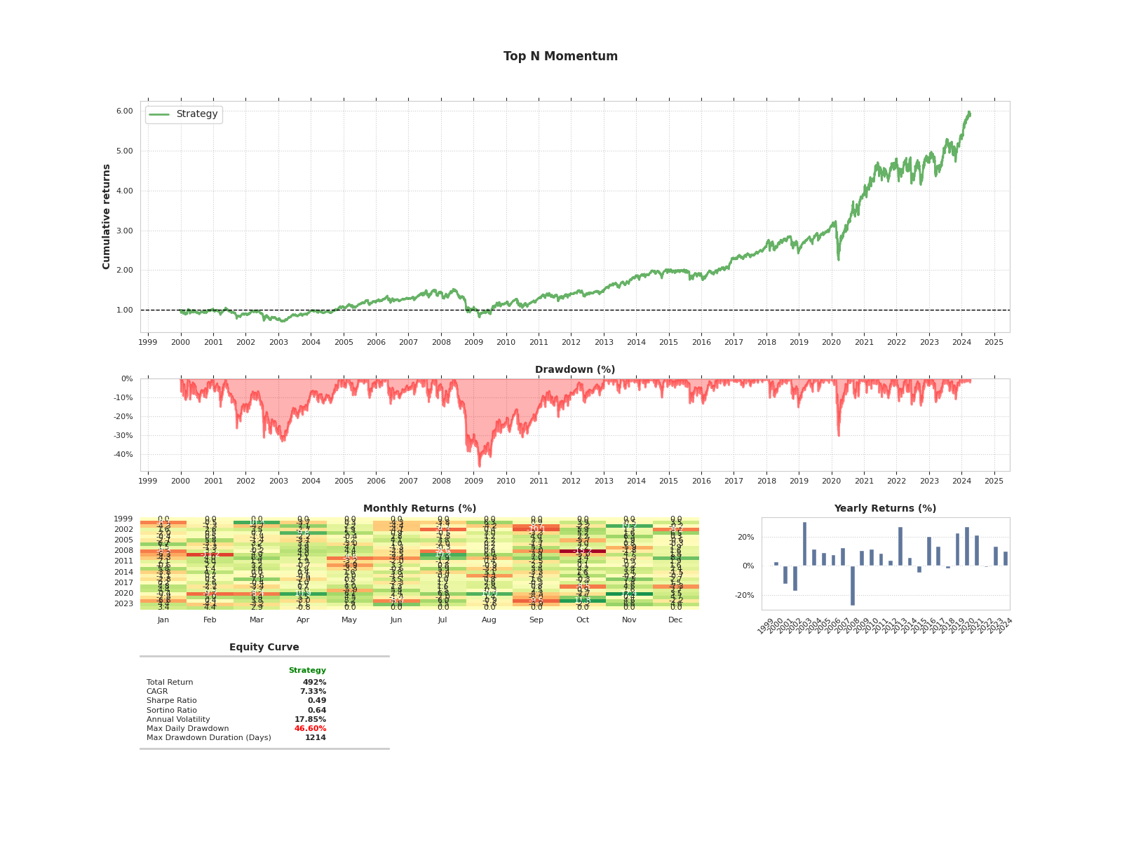
You can now run the backtest in your Jupyter environment. To plot and save the tearsheet all you need to do is add the following lines of code to a new cell.

# Performance Output
tearsheet = TearsheetStatistics(
    strategy_equity=strategy_backtest.get_equity_curve(),
    title='Top N Momentum'
)
tearsheet.plot_results(filename='TopNMomentum_tearsheet.png') 

The tearsheet will be saved in the qst_startdev_notebooks directory and should also be visible in the notebook.

We hope that this tutorial has given you some insight into the avaiable components inside QSTrader, as well as an overview of how to put them all together in order to build and run new strategies. Using the backtesting environment created in the last two tutorials will allow you to explore QSTrader as well as extend the framework for your own requirements.