In this tutorial we will set up a backtesting environment which uses the QSTrader backtesting framework inside a Jupyter Notebook. We will isolate this research environment and it's dependencies using Docker, with Docker Compose. In the next article we will show you how to implement one of the example strategies for QSTrader, the Momentum Top N tactical asset allocation strategy. In order to follow along with this tutorial you will need to have pre-installed Docker and Docker Compose. The Docker website has some excellent platform specific tutorials that will allow you to get up and running with both.

The Jupyter Notebook interface allows users to create and share documents that contain live code, equations, visualizations, and narrative text. This aids in the development and optimisation of strategies by offering built-in data visualisations, allowing you to quickly iterate through different variables in your backtests and easily compare the changes by examining the tearsheets.

Using containers, like Docker, allows developers to package an application with all of its dependencies into a single standardized unit of software. This makes it possible for applications to run consistently across any environment, whether on a local laptop, a test server, or in the cloud. Docker also supports CI/CD (Continuous Integration/Continuous Deployment), allowing developers to quickly build, test, and deploy applications with minimal overhead and variability between environments.

If you wish to understand more about Docker their website has some excellent resources including:

• Quick hands-on guides which allow you to gain specific knowledge no matter your starting point.
• Complete guide for those at the beginning of their docker journey.
• Docker concepts video series for visual learners.
• Creating a container from scratch an excellent video which explains how containers are created and isolated. Worth a watch for those who are curious about what happens 'underneath'!

Setting up the directory structure

There is no right or wrong way to set up a directory structure for dockerised applications, although it is generally better to adhere to the best practices of software development. Below we suggest a method that is modular, scalable and maintainable.

The application we are creating here, which we have called qstrader-notebooks, contains subdirectories for orchestration and components. Organising directories by components allows developers to isolate functionality into distinct, manageable pieces. Each component can be developed, tested, and deployed independently, which simplifies updates and debugging. This modularity also supports the principles of microservices architectures, where each service is encapsulated in its own container. This allows developers to add more components easily with Dockerfiles contained inside each additional service.

The orchestration directory will contain the docker-compose.yml file to orchestrate our services, networks and volumes. Keeping orchestration scripts (like Docker Compose files or Kubernetes YAML configurations) in separate directories aids in the deployment and management aspects of applications. This separation ensures that operational configurations are not mixed with application logic, making it easier to deploy across different environments.

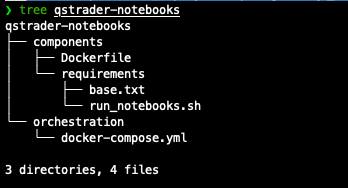
In addition to the Dockerfile and docker-compose.yml file we also have a requirements directory containing base.txt and run_notebooks.sh. Base.txt will contain our dependencies QSTrader and Jupyter Notebooks. Run_notebooks.sh is a shell script which will be executed once the docker container has been initalised and will activate Jupyter Notebook. The rest of the tutorial will assume this directory structure has been followed and will implement some path specific context inside the docker-compose.yml. If you are unsure how to modify the paths we suggest you follow the structure as defined here, otherwise feel free to edit the paths to fit the directory structure of your choosing.

Initialising Docker and Docker Compose

Once you have created the directories and files required we can start to create our Dockerfile. To initialise our Docker container we can add the following to the Dockerfile.

    # Pull Base Image
    FROM ubuntu:22.04

    # Set environment variables
    ENV PYTHONDONTWRITEBYTECODE 1
    ENV PYTHONUNBUFFERED 1
    ENV TZ=Europe/London
    RUN ln -snf /usr/share/zoneinfo/$TZ /etc/localtime && echo $TZ > /etc/timezone

    # Update and Upgrade
    RUN apt-get update -y && apt-get upgrade -y

    # Add base sysadmin/coding tools
    RUN apt-get install -y build-essential vim python3-dev python3-pip

    # Set the work directory
    WORKDIR /app

We start by pulling in a Ubuntu base image. We have chosen to use the full Ubuntu image rather than a lightweight version like Ubuntu Base, as it comes with more of the utilities necessary to run certain programmes. As we plan to visualise equity curves of our strategies this choice will give us access to all of the underlying packages required. For those interested in how to choose an appropriate base image for your Dockerfile there is an excellent article here.

After selecting the base image we can set up our environment variables. These are prefixed with ENV instructing docker to set an environemnt variable that will be available at all subsequent stages of the build process.

• PYTHONWRITEBYTECODE 1: This prevents Python from writing .pyc files. Inside a container invocations of Python programs and dependencies occurs once so it is usually not neccessary to store the byte code. If, however, mulitple Python processes are spawned it might be more efficient to store the .pyc files.
• PYTHONUNBUFFERED 1: This forces the stderr and stdout streams to be unbuffered, which benefits debugging in the Docker log. When the streams are buffered text output and error messages can be retained in the buffer and duplicated in the output, making the logs harder to read.
• TZ=Europe/London: As we are using time series data for backtesting the correct time zone should be set. Please set this according to your loaction.

Now we can RUN a command to update the timezone setting on our base image. We update and upgarde all the packages provided by the base image and install build-essential, vim and Python3 with pip3. The final command WORKDIR sets the working directory for our project to be /app. This is were any subsequent RUN, CMD, ENTRYPOINT, COPY and ADD instructions will be run from. Once the container is active you will be able to navigte to /app and see the requirements folder which is added to the Dockerfile in the next section.

With the Dockerfile started we can set up the docker-compose.yml and we will be able to create our initial Docker container. Add the following to the docker-compose.yml file inside the orchestration subdirectory.

services:
  qst:
    build:
      context: ../components
    volumes:
      - ../qst_stratdev_notebooks:/app/notebooks
      - ../qst_stratdev_data:/data
    ports:
     - 8888:8888

We start by specifying our services, which we name qst as an abbreviation for QSTrader. We give our Compose file a build specification with a context path. This will be used to execute the build and Docker will look for a Dockerfile in this directory. The path can be absolute or, as shown above, it can be relative to the location of your docker-compose.yml file.

Next we need to define a two volumes for our service. Volumes are persistent data stores which are implemented by Docker. They can be used across multiple services and Compose offers many options for configuration. Here we have defined separate volume mounts for our notebooks and for the time series data associated with the strategies. For simplicity we have created a notebooks and data directory inside the root of our application. However, these paths can be adjusted as you wish. At the end of the path we map the host location to the container location with a colon. Our notebooks directory will be visible under /app inside the container and the data directory will be located at the root of the container. This design choice is useful if you are using vesion control, such as git and wish to keep your data outside of your application repository.

Finally we map the ports between the host and the container. This will allow us to visualise the notebooks through the browser on the host machine by navigating to localhost:/8888. Port 8888 is the unofficially reserved port for Ipython and Jupyter Notebooks. To find out more about reserved ports check out this article.

Before we build our container for the first time there is one more line that we can add to our Dockerfile. The tail command outputs the last 10 lines of a file to stdout, the -f flag means append or do this continuously. This is then written to /dev/null, a 'blackhole'. It has the effect of keeping the container active, allowing us to access it and look around inside, before we try to get Jupyter Notebooks up and running. Once the Dockerfile is complete we will remove this line. For now add the following to the end of the Docker file:

CMD tail -f /dev/null

We can now build our Docker container by navigating to the orchestration directory and typing docker compose up --build -d into your terminal. The -d flag detatches the process so it runs in the background and returns control of the terminal. This will take a while to build initially as you will have to create the Ubuntu image. In Subsequent activations of the container we will omit the --build flag and Docker will use the cache, speeding up the process.

Once the contatiner has built you can type docker ps and you should see the container listed. The name of the container will be under NAMES. The container can be accessed by typing docker exec --it CONTAINER-NAME /bin/bash into your terminal, remembering to substitute in the name of the container on your system.

Once inside you can navigate around as you would normally inside a terminal. Typing ls should show you that you have the notebooks directory present, as defined in our docker-compose.yml.

When you have finished you can simply exit the container by typing exit. You can shut down the container by navigating to the orchestration directory and typing docker compose down. This will gracefully exit the Docker container, ready for us to add Jupyter Notebooks and QSTrader to the build.

Installing the dependencies

We can now specify our package requirements such that they will be incorporated into the build process of our container. Add the following to base.txt inside the components/reuirements/subdirectory.

qstrader==0.2.6
notebook==7.1

Now we need to copy the file across to our container and run pip install. In the Dockerfile add the following lines above the CMD tail -f /dev/null line:

# Install dependencies
COPY requirements/base.txt /app/
RUN pip3 install -r base.txt

Now we can build the Docker container again by navigating to orchestration and typing docker compose up -d. You should notice that the first five steps of the build process are cached. Once complete you can access the system by typing docker exec --it CONTAINER-NAME /bin/bash. Once inside you can type pip3 freeze | grep qstrader you should see qstrader version 0.2.6 listed in the output.

Activate notebooks within Dockerfile

You now have QSTrader and Jupyter Notebooks installed in a Docker container. You can activate Jupyter Notebook using the following command:

jupyter notebook --ip 0.0.0.0 --no-browser --allow-root --NotebookApp.token=''

Lets take a look as the optional flags in this command:

• --ip 0.0.0.0 configures the notebook server to listen on all IPs.
• --no-browser tells Jupyter Notebook not to open a browser window.
• --allow-root gives you root access.
• --NotebookApp.token='' replaces the password with a blank string.

Note that running as root inside the Docker container and Jupyter Notebook, as well as disabling the password token for Jupyter are NOT best practice. However, as we are running Docker on our own host machine and not in a wider setting this is an exceptable trade off. If you decide to transfer your qst-notebook application to be used as part of a larger scale system, you will need to review the security options.

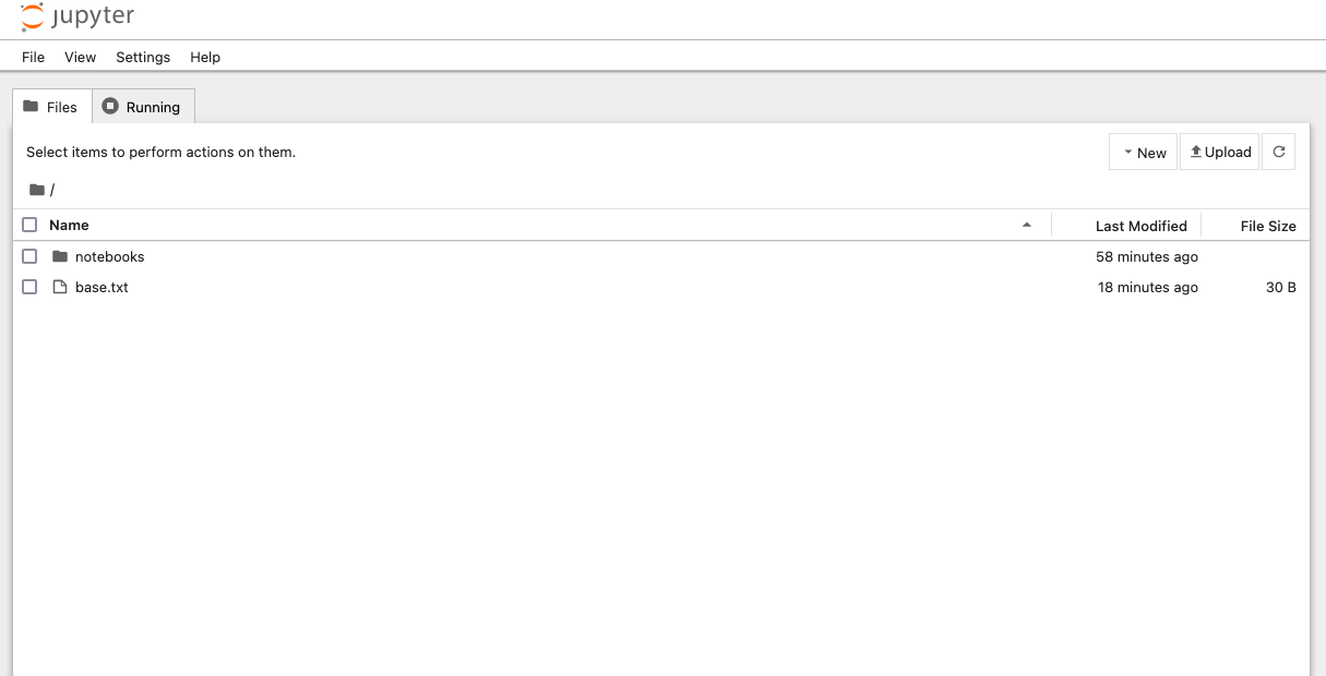
After typing this command into the Docker container you can visualise the Jupyter Notebooks in the browser on your host machine by navigating to localhost:/8888. You should see the familiar Jupyter notebooks menu.

You can automate the activation of Jupyter Notebook by creating a shell script which can be executed during the container build. Exit the container and shut it down as before using docker compose down. In components/requirements/ edit the run_notebooks.sh file to include the jupyter notebook command we used above. You will need to add the tail -f /dev/null command to redirect the output to dev/null and keep the container running. Add the following command to run_notebooks.sh:

jupyter notebook --ip 0.0.0.0 --no-browser --allow-root --NotebookApp.token='' && tail -f /dev/null

Now we can edit the Dockerfile to copy across the shell script, make it executable and run it to activate Jupyter Notebooks. Add the following to the Dockerfile and remove the final line CMD tail -f /dev/null.

# Run notebooks
COPY requirements/run_notebooks.sh /app/
RUN chmod +x /app/run_notebooks.sh

CMD ./run_notebooks.sh

You can now rebuild the container with docker compose up -d and you should be able to access your notebook environment in the browser of you host machine by navigating to localhost/:8888.

This concludes the first of two tutorials; the creation of a backtesting research environment. In the next article we will be implementing an example strategy using the QSTrader backtesting framework. We will be using Momentum Top N, a tactical assest allocation strategy, from the QSTrader examples.