Tutorial: Momentum Tactical Asset Allocation Strategy
In the previous tutorial we considered a simple static allocation portfolio with periodic rebalancing. In this tutorial we are going to create a backtest on a well-known dynamic tactical asset allocation strategy known as sector momentum.
Much of the code will be similar to the previous tutorial but we will introduce some new features. We will add the DynamicUniverse class, which allows us to change the potential asset composition through time. We will describe the MomentumSignal and SignalsCollection entities that pre-calculate the momentum time series for us. We will also describe how to build a custom AlphaModel to generate specific signals to feed into the portfolio optimisation process.
As with the previous tutorial this tutorial assumes you have correctly installed QSTrader.
Please note that all of the code below can be found within the /examples/momentum_taa.py file at the QSTrader GitHub repository. We will be referring to this file in the tutorial steps below.
The first task is to either download the momentum_taa.py file, utilise the full code at the end of this tutorial or create a new empty file to type in the code below manually.
We will begin by describing the strategy and download the necessary data from Yahoo Finance. We will subsequently describe all code in momentum_taa.py and finally execute the backtest to display a performance 'tearsheet'.
Strategy Explanation
The US sector momentum strategy is a long-only dynamic tactical asset allocation strategy that attempts to exceed the performance of simply going long the S&P500.
At the end of every month the strategy calculates the holding period return (HPR) based momentum of all of the SPDR sector ETFs (the ticker symbols of which begin with the prefix XL) and selects the top N to invest in for the forthcoming month, where N is usually between 3 and 6.
In the implementation given here the HPR momentum is calculated over the previous 126 days (approximately six months of business days) and the top three sector ETFs are chosen for the portfolio. The portfolio allocation is equally weighted between each of these three sector ETFs. Irrespective of changes in signal the portfolio is rebalanced once per month to weight the assets equally.
QSTrader automatically provides functionality for calculating the momentum values of each asset. The code presented below thus concentrates on the strategy logic of determining the highest momentum assets and then weighting them equally.
Downloading the Data
The momentum_taa.py code makes use of OHLC 'daily bar' data from Yahoo Finance. In particular it requires the following SPDR sector ETFs: XLB, XLC, XLE, XLF, XLI, XLK, XLP, XLU, XLV and XLY. For example, XLK can be downloaded here. Download the full history for each and save as CSV files in same directory as momentum_taa.py.
Defining a Backtest Script
Much of the code below is similar to that outlined in the previous tutorial but for completeness we will explain all code from scratch and include the full code at the end of this tutorial.
Note: The full code below contains extensive comments in order to fully qualify the parameters and return types. Some of these comments have been removed in the snippets as the tutorial progresses to enhance readability.
Module Imports
The first part of the Python code imports the necessary modules from within the QSTrader library:
# momentum_taa.py

import operator
import os

import pandas as pd
import pytz

from qstrader.alpha_model.alpha_model import AlphaModel
from qstrader.alpha_model.fixed_signals import FixedSignalsAlphaModel
from qstrader.asset.equity import Equity
from qstrader.asset.universe.dynamic import DynamicUniverse
from qstrader.asset.universe.static import StaticUniverse
from qstrader.signals.momentum import MomentumSignal
from qstrader.signals.signals_collection import SignalsCollection
from qstrader.data.backtest_data_handler import BacktestDataHandler
from qstrader.data.daily_bar_csv import CSVDailyBarDataSource
from qstrader.statistics.tearsheet import TearsheetStatistics
from qstrader.trading.backtest import BacktestTradingSession
We first import operator as this is needed to select the top performing momentum assets. We also import os as we need to query the environment for the appropriate QSTrader data directory. It is possible to tell QSTrader to look for data in a directory other than the same directory as the momentum_taa.py file, but for the purposes of this tutorial we will assume the data will eventually be stored in the same directory.
We then import Pandas and Pytz, which are needed for handling timestamp functionality with timezones.
The remaining imports are within QSTrader itself. We first import the AlphaModel abstract base class, which will be used to create our momentum alpha model sub class. We also import FixedSignalsAlphaModel for the S&P500 benchmark.
An AlphaModel in QSTrader terms is a class that emits a dimensionless 'forecast' or 'signal' for a particular collection of assets (known as an 'asset universe').
The FixedSignalsAlphaModel is a simple signal generator that emits constant forecasts, irrespective of market behaviour for a particular collection of assets. As we are going to compare the momentum TAA strategy against buying and holding the S&P500 we need a fixed signal of 1.0 for the SPY ETF, which represents this benchmark.
We import Equity in order to tell the module that loads the data from CSV files that the CSV files represent equity prices/volumes.
We import both the StaticUniverse and DynamicUniverse classes. Our momentum asset 'universe' consists of a time-varying collection. XLC (representing the 'communications' sector) was added more recently compared to the other nine sector ETFs. Hence we need to use the DynamicUniverse class to tell QSTrader that a new asset is added during the backtest period. The StaticUniverse class is used for the static buy and hold benchmark of SPY.
The main difference between this tutorial and the previous tutorial is the inclusion of MomentumSignal and SignalsCollection. These are helper classes that calculate the momentum on a collection of assets, for a collection of lookback periods. We will discuss these in more detail below.
We import the helper BacktestDataHandler class that determines how our asset universe specification and data source(s) are linked.
We import the CSVDailyBarDataSource because the particular data sources used within this tutorial are CSV files, as opposed to a database, web URL or file store (such as HDF5).
Since we wish to visualise our backtest results we want to import the TearsheetStatistics class.
Finally to tie it all together we import the BacktestTradingSession, which runs our scheduled backtest 'engine' between the specified start and end timestamps.
Momentum Alpha Model Definition
Another difference between this and the previous tutorial is that we are creating our own AlphaModel logic via the TopNMomentumAlphaModel class. This is where most of the strategy logic is contained:
# momentum_taa.py

class TopNMomentumAlphaModel(AlphaModel):

    def __init__(
        self, signals, mom_lookback, mom_top_n, universe, data_handler
    ):
        self.signals = signals
        self.mom_lookback = mom_lookback
        self.mom_top_n = mom_top_n
        self.universe = universe
        self.data_handler = data_handler

        def _highest_momentum_asset(
            self, dt
        ):
            assets = self.signals['momentum'].assets

            # Calculate the holding-period return momenta for each asset,
            # for the particular provided momentum lookback period
            all_momenta = {
                asset: self.signals['momentum'](
                    asset, self.mom_lookback
                ) for asset in assets
            }

            # Obtain a list of the top performing assets by momentum
            # restricted by the provided number of desired assets to
            # trade per month
            return [
                asset[0] for asset in sorted(
                    all_momenta.items(),
                    key=operator.itemgetter(1),
                    reverse=True
                )
            ][:self.mom_top_n]

        def _generate_signals(
            self, dt, weights
        ):
            top_assets = self._highest_momentum_asset(dt)
            for asset in top_assets:
                weights[asset] = 1.0 / self.mom_top_n
            return weights

        def __call__(
            self, dt
        ):
            assets = self.universe.get_assets(dt)
            weights = {asset: 0.0 for asset in assets}

            # Only generate weights if the current time exceeds the
            # momentum lookback period
            if self.signals.warmup >= self.mom_lookback:
                weights = self._generate_signals(dt, weights)
            return weights
We can see that the class takes five parameters.
It takes a SignalsCollection instance so that is has access to pre-computed momentum signals.
It takes two momentum related parameters: mom_lookback and mom_top_n. The first is the integer number of business days to calculate holding period return (HPR) momentum over. The second determines how many assets to trade in a particular month.
It also takes in a Universe instance (in this case our DynamicUniverse described above) and a DataHandler to get underlying access to the pricing data.
The first method is _highest_momentum_asset. It obtains the momentum signals on all current assets, for the particular specified lookback period, and places these into a dictionary keyed by the asset symbol. It then utilises the Python sorted built-in function, along with the operator.itemgetter method and a list comprehension to create a reverse-ordered list of highest momentum assets, slicing this list to the top N assets.
For example, the output of this list might look like ['EQ:XLC', 'EQ:XLB', 'EQ:XLK'] if these were the top three highest momentum assets within this period.
The second method is _generate_signals. It simply calls the _highest_momentum_asset method and produces a weights dictionary with each of these assets weighted equally.
For example, the output might look like {'EQ:XLC': 0.3333333, 'EQ:XLB': 0.3333333, 'EQ:XLK': 0.3333333}.
The final method, turning the TopNMomentumAlphaModel into a callable, is __call__. This wraps the other two previous methods and only generates these weights if enough data has been collected at this point in the backtest to generate a full lookback momentum signal for each asset. Finally, the weights dictionary is returned.
We will use an instance of this class in the if __name__ == "__main__": entry point below.
Backtest Duration
The next task is to define the script entry point and specify when the backtest runs from and to. Another difference between this tutorial and the previous tutorial is that we now need to specify a 'burn in' time. This differs from the start time of the backtest:
# momentum_taa.py

if __name__ == "__main__":
    # Duration of the backtest
    start_dt = pd.Timestamp('1998-12-22 14:30:00', tz=pytz.UTC)
    burn_in_dt = pd.Timestamp('1999-12-22 14:30:00', tz=pytz.UTC)
    end_dt = pd.Timestamp('2020-12-31 23:59:00', tz=pytz.UTC)
The burn in time is the time at which weights are actually generated and sent to the portfolio construction instance. This is necessary because the momentum HPR signal has a lookback period. If insufficient daily data exists at a particular point in the backtest we have chosen not to generate signals until data becomes available.
Note: The dates make use of the Pandas Timestamp class and require timezone specification via pytz.
Note: An alternative approach is to use an expanding window lookback period that makes use of whatever data is curently available to calculate a momentum signal up until sufficient data exists to utilise the full lookback period. We have chosen to not use expanding windows in this tutorial.
Note: At this stage of QSTrader development, for the 'buy & hold' methodology used below in the benchmark calculation it is necessary to specify a starting time of 14:30:00 UTC in order for the backtest to proceed correctly.
Model Parameters
The top N momentum model requires two parameters. The first is the total number of business days to use in the HPR momentum signal. In this tutorial we have chosen 126, which is approximately six months worth of business days. The second parameter is the number of assets to include in the (equally weighted) portfolio every month.
# momentum_taa.py

    # Model parameters
    mom_lookback = 126  # Six months worth of business days
    mom_top_n = 3  # Number of assets to include at any one time
Asset Universe
The next task is to construct the dynamic asset universe for the backtest:
# momentum_taa.py

    # Construct the symbols and assets necessary for the backtest
    # This utilises the SPDR US sector ETFs, all beginning with XL
    strategy_symbols = ['XL%s' % sector for sector in "BCEFIKPUVY"]
    assets = ['EQ:%s' % symbol for symbol in strategy_symbols]

    # As this is a dynamic universe of assets (XLC is added later)
    # we need to tell QSTrader when XLC can be included. This is
    # achieved using an asset dates dictionary
    asset_dates = {asset: start_dt for asset in assets}
    asset_dates['EQ:XLC'] = pd.Timestamp('2018-06-18 00:00:00', tz=pytz.UTC)
    strategy_universe = DynamicUniverse(asset_dates)
QSTrader requires that the assets are prefixed with a two letter code describing their instrument type. In this simulation the assets must be prefixed with EQ, representing equity-like (common stock and ETFs) instruments.
The first task is to create an assets list that contains all ten ETFs used in the backtest. The next task is to construct an asset_dates dictionary that is keyed on the asset symbol and contains the starting date for each asset in the dynamic universe. All but one of the ETFs begin on the start date of the backtest, however XLC starts on June 18th 2018 and its starting date is modified accordingly.
The asset_dates dictionary is passed into the DynamicUniverse instance to create the universe of assets for the strategy backtest.
Pricing Data
The next task is to obtain the appropriate data for these symbols and load it into the data handler:
# momentum_taa.py

    # To avoid loading all CSV files in the directory, set the
    # data source to load only those provided symbols
    csv_dir = os.environ.get('QSTRADER_CSV_DATA_DIR', '.')
    strategy_data_source = CSVDailyBarDataSource(csv_dir, Equity, csv_symbols=strategy_symbols)
    strategy_data_handler = BacktestDataHandler(strategy_universe, data_sources=[strategy_data_source])
Firstly we determine the appropriate data directory if it has been set externally by the environment, otherwise we default to the same directory as momentum_taa.py. Then we load the CSV data and tie it together with the asset universe through a BacktestDataHandler.
Signals
In this section of momentum_taa.py we create the MomentumSignal helper class, passing the universe we wish to calculate momentum on, as well as the range of lookbacks we are interested in. Since we are only interested in one lookback period we only include a single item list of [mom_lookback].
The SignalsCollection is used to wrap the various signals we may be using within our alpha model instances. For the purposes of this tutorial we are only using momentum signals so we pass this in as a single element dictionary:
# momentum_taa.py

    # Generate the signals (in this case holding-period return based
    # momentum) used in the top-N momentum alpha model
    momentum = MomentumSignal(start_dt, strategy_universe, lookbacks=[mom_lookback])
    signals = SignalsCollection({'momentum': momentum}, strategy_data_handler)
Alpha Model and Backtest
The next set of code instantiates the top N momentum alpha model defined earlier, creates the backtest instance and executes it:
# momentum_taa.py

    # Generate the alpha model instance for the top-N momentum alpha model
    strategy_alpha_model = TopNMomentumAlphaModel(
        signals, mom_lookback, mom_top_n, strategy_universe, strategy_data_handler
    )

    # Construct the strategy backtest and run it
    strategy_backtest = BacktestTradingSession(
        start_dt,
        end_dt,
        strategy_universe,
        strategy_alpha_model,
        signals=signals,
        rebalance='end_of_month',
        long_only=True,
        cash_buffer_percentage=0.01,
        burn_in_dt=burn_in_dt,
        data_handler=strategy_data_handler
    )
    strategy_backtest.run()
Note the addition of both the signals and burn_in_dt keyword arguments, which are not required in the previous tutorial.
Firstly the TopNMomentumAlphaModel is initialised with the parameters that have been defined above.
Subsequently the BacktestTradingSession is initialised with the starting, burn-in and ending dates, the dynamic asset universe, the signals collection and the particular alpha model defined above.
In addition it is necessary to supply a rebalance keyword argument. This tells the QSTrader backtesting engine how frequently to re-run the signal generation and portfolio construction logic. Since this is decoupled from the actual data timestamps it is necessary to be explicit about how frequently this is carried out.
For this particular strategy we are going to carry out the signal generation and portfolio construction once per month at the close of the final trading day. This means that if the true percentage allocations of each sector ETF have drifted from their equal weight allocations across the month some additional 'rebalance' trades will be issued to buy/sell the appropriate amount of the ETFs in order to bring the account allocations inline with these targets.
The long_only keyword argument lets the backtester know that this strategy only goes 'long' (that is, does not borrow and 'short' any assets on margin).
We also require a 'cash buffer' in the account in order to handle the case where a target order for a particular quantity of stock is generated (at market close) but when executed at the next market open the order is found to be too expensive for the current account equity to execute.
This can occur if the stock price for this asset has jumped up significantly overnight. This cash buffer attempts to account for such jumps. It maintains this (approximate) percentage of the account equity in cash to cover this eventuality. We have set it to 1% of account equity here but it may be necessary to modify this value if backtesting on particularly volatile equities.
Finally we tell the backtesting engine which data handler to use and execute the backtest with the run method.
At this stage, once the backtest has finished executing the strategy_backtest instance contains all of the calculated values of the backtest (such as the equity curve, drawdown curve and various other statistics).
Benchmark
However we are also interested in comparing this result to another 'benchmark' strategy, which is simply a 'buy & hold' of the SPY ETF. This allows to see what has happened over the backtest duration if we simply held onto an ETF representing the US S&P500 during this time period instead.
To create a benchmark we run another full backtest but on a different alpha model and rebalance schedule:
# momentum_taa.py

    # Construct benchmark assets (buy & hold SPY)
    benchmark_symbols = ['SPY']
    benchmark_assets = ['EQ:SPY']
    benchmark_universe = StaticUniverse(benchmark_assets)
    benchmark_data_source = CSVDailyBarDataSource(csv_dir, Equity, csv_symbols=benchmark_symbols)
    benchmark_data_handler = BacktestDataHandler(benchmark_universe, data_sources=[benchmark_data_source])

    # Construct a benchmark Alpha Model that provides
    # 100% static allocation to the SPY ETF, with no rebalance
    benchmark_alpha_model = FixedSignalsAlphaModel({'EQ:SPY': 1.0})
    benchmark_backtest = BacktestTradingSession(
        burn_in_dt,
        end_dt,
        benchmark_universe,
        benchmark_alpha_model,
        rebalance='buy_and_hold',
        long_only=True,
        cash_buffer_percentage=0.01,
        data_handler=benchmark_data_handler
    )
    benchmark_backtest.run()
Note that the FixedSignalsAlphaModel has a 100% allocation to SPY for the benchmark. It also uses the 'buy_and_hold' rebalance schedule. The latter informs the backtester to generate a single signal at the beginning of the backtest to go fully long SPY. There are no further trades carried out for the benchmark.
The remaining parameters are similar and we run the benchmark backtest once again with the run method.
Note: The 'start date' has been replaced with the burn_in_dt from above. This is because this is the first date that trades are calculated for the momentum strategy. In order to compare 'apples to apples' it is necessary to start the benchmark from this point also.
Tearsheet
All of the backtest results are now stored in strategy_backtest and benchmark_backtest. However we would like to visualise these results and output some basic statistics. For this we can use a 'tearsheet':
# momentum_taa.py

    # Performance Output
    tearsheet = TearsheetStatistics(
        strategy_equity=strategy_backtest.get_equity_curve(),
        benchmark_equity=benchmark_backtest.get_equity_curve(),
        title='US Sector Momentum - Top 3 Sectors'
    )
    tearsheet.plot_results()
The TearsheetStatistics class is instantiated with the strategy backtest equity curve, the (optional) benchmark backtest equity curve and a supplied title. Finally the results are plotted (using Matplotlib) through the plot_results method.
Executing the Backtest
To run the code ensure that your Python virtual environment, such as Anaconda or virtualenv is activated. Then type the following in the same directory as momentum_taa.py:
python momentum_taa.py
You will see both the strategy and benchmark backtests being calculated. Finally the tearsheet will appear depicting the results. It should look like the following:
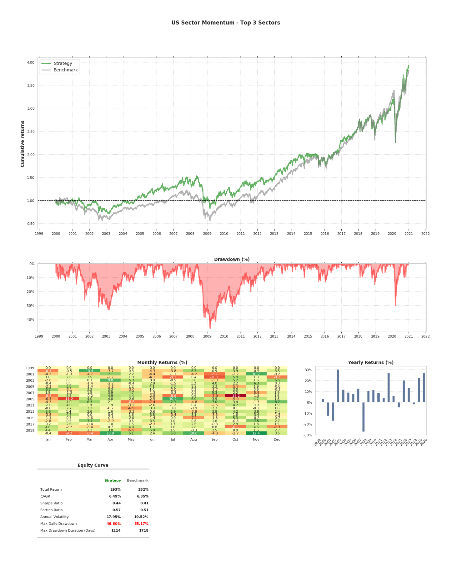
You have now successfully completed your first QSTrader momentum tactical asset allocation strategy backtest!
Full Code
# momentum_taa.py

import operator
import os

import pandas as pd
import pytz

from qstrader.alpha_model.alpha_model import AlphaModel
from qstrader.alpha_model.fixed_signals import FixedSignalsAlphaModel
from qstrader.asset.equity import Equity
from qstrader.asset.universe.dynamic import DynamicUniverse
from qstrader.asset.universe.static import StaticUniverse
from qstrader.signals.momentum import MomentumSignal
from qstrader.signals.signals_collection import SignalsCollection
from qstrader.data.backtest_data_handler import BacktestDataHandler
from qstrader.data.daily_bar_csv import CSVDailyBarDataSource
from qstrader.statistics.tearsheet import TearsheetStatistics
from qstrader.trading.backtest import BacktestTradingSession


class TopNMomentumAlphaModel(AlphaModel):

    def __init__(
        self, signals, mom_lookback, mom_top_n, universe, data_handler
    ):
        """
        Initialise the TopNMomentumAlphaModel

        Parameters
        ----------
        signals : `SignalsCollection`
            The entity for interfacing with various pre-calculated
            signals. In this instance we want to use 'momentum'.
        mom_lookback : `integer`
            The number of business days to calculate momentum
            lookback over.
        mom_top_n : `integer`
            The number of assets to include in the portfolio,
            ranking from highest momentum descending.
        universe : `Universe`
            The collection of assets utilised for signal generation.
        data_handler : `DataHandler`
            The interface to the CSV data.

        Returns
        -------
        None
        """
        self.signals = signals
        self.mom_lookback = mom_lookback
        self.mom_top_n = mom_top_n
        self.universe = universe
        self.data_handler = data_handler

    def _highest_momentum_asset(
        self, dt
    ):
        """
        Calculates the ordered list of highest performing momentum
        assets restricted to the 'Top N', for a particular datetime.

        Parameters
        ----------
        dt : `pd.Timestamp`
            The datetime for which the highest momentum assets
            should be calculated.

        Returns
        -------
        `list[str]`
            Ordered list of highest performing momentum assets
            restricted to the 'Top N'.
        """
        assets = self.signals['momentum'].assets

        # Calculate the holding-period return momenta for each asset,
        # for the particular provided momentum lookback period
        all_momenta = {
            asset: self.signals['momentum'](
                asset, self.mom_lookback
            ) for asset in assets
        }

        # Obtain a list of the top performing assets by momentum
        # restricted by the provided number of desired assets to
        # trade per month
        return [
            asset[0] for asset in sorted(
                all_momenta.items(),
                key=operator.itemgetter(1),
                reverse=True
            )
        ][:self.mom_top_n]

    def _generate_signals(
        self, dt, weights
    ):
        """
        Calculate the highest performing momentum for each
        asset then assign 1 / N of the signal weight to each
        of these assets.

        Parameters
        ----------
        dt : `pd.Timestamp`
            The datetime for which the signal weights
            should be calculated.
        weights : `dict{str: float}`
            The current signal weights dictionary.

        Returns
        -------
        `dict{str: float}`
            The newly created signal weights dictionary.
        """
        top_assets = self._highest_momentum_asset(dt)
        for asset in top_assets:
            weights[asset] = 1.0 / self.mom_top_n
        return weights

    def __call__(
        self, dt
    ):
        """
        Calculates the signal weights for the top N
        momentum alpha model, assuming that there is
        sufficient data to begin calculating momentum
        on the desired assets.

        Parameters
        ----------
        dt : `pd.Timestamp`
            The datetime for which the signal weights
            should be calculated.

        Returns
        -------
        `dict{str: float}`
            The newly created signal weights dictionary.
        """
        assets = self.universe.get_assets(dt)
        weights = {asset: 0.0 for asset in assets}

        # Only generate weights if the current time exceeds the
        # momentum lookback period
        if self.signals.warmup >= self.mom_lookback:
            weights = self._generate_signals(dt, weights)
        return weights


if __name__ == "__main__":
    # Duration of the backtest
    start_dt = pd.Timestamp('1998-12-22 14:30:00', tz=pytz.UTC)
    burn_in_dt = pd.Timestamp('1999-12-22 14:30:00', tz=pytz.UTC)
    end_dt = pd.Timestamp('2020-12-31 23:59:00', tz=pytz.UTC)

    # Model parameters
    mom_lookback = 126  # Six months worth of business days
    mom_top_n = 3  # Number of assets to include at any one time

    # Construct the symbols and assets necessary for the backtest
    # This utilises the SPDR US sector ETFs, all beginning with XL
    strategy_symbols = ['XL%s' % sector for sector in "BCEFIKPUVY"]
    assets = ['EQ:%s' % symbol for symbol in strategy_symbols]

    # As this is a dynamic universe of assets (XLC is added later)
    # we need to tell QSTrader when XLC can be included. This is
    # achieved using an asset dates dictionary
    asset_dates = {asset: start_dt for asset in assets}
    asset_dates['EQ:XLC'] = pd.Timestamp('2018-06-18 00:00:00', tz=pytz.UTC)
    strategy_universe = DynamicUniverse(asset_dates)

    # To avoid loading all CSV files in the directory, set the
    # data source to load only those provided symbols
    csv_dir = os.environ.get('QSTRADER_CSV_DATA_DIR', '.')
    strategy_data_source = CSVDailyBarDataSource(csv_dir, Equity, csv_symbols=strategy_symbols)
    strategy_data_handler = BacktestDataHandler(strategy_universe, data_sources=[strategy_data_source])

    # Generate the signals (in this case holding-period return based
    # momentum) used in the top-N momentum alpha model
    momentum = MomentumSignal(start_dt, strategy_universe, lookbacks=[mom_lookback])
    signals = SignalsCollection({'momentum': momentum}, strategy_data_handler)

    # Generate the alpha model instance for the top-N momentum alpha model
    strategy_alpha_model = TopNMomentumAlphaModel(
        signals, mom_lookback, mom_top_n, strategy_universe, strategy_data_handler
    )

    # Construct the strategy backtest and run it
    strategy_backtest = BacktestTradingSession(
        start_dt,
        end_dt,
        strategy_universe,
        strategy_alpha_model,
        signals=signals,
        rebalance='end_of_month',
        long_only=True,
        cash_buffer_percentage=0.01,
        burn_in_dt=burn_in_dt,
        data_handler=strategy_data_handler
    )
    strategy_backtest.run()

    # Construct benchmark assets (buy & hold SPY)
    benchmark_symbols = ['SPY']
    benchmark_assets = ['EQ:SPY']
    benchmark_universe = StaticUniverse(benchmark_assets)
    benchmark_data_source = CSVDailyBarDataSource(csv_dir, Equity, csv_symbols=benchmark_symbols)
    benchmark_data_handler = BacktestDataHandler(benchmark_universe, data_sources=[benchmark_data_source])

    # Construct a benchmark Alpha Model that provides
    # 100% static allocation to the SPY ETF, with no rebalance
    benchmark_alpha_model = FixedSignalsAlphaModel({'EQ:SPY': 1.0})
    benchmark_backtest = BacktestTradingSession(
        burn_in_dt,
        end_dt,
        benchmark_universe,
        benchmark_alpha_model,
        rebalance='buy_and_hold',
        long_only=True,
        cash_buffer_percentage=0.01,
        data_handler=benchmark_data_handler
    )
    benchmark_backtest.run()

    # Performance Output
    tearsheet = TearsheetStatistics(
        strategy_equity=strategy_backtest.get_equity_curve(),
        benchmark_equity=benchmark_backtest.get_equity_curve(),
        title='US Sector Momentum - Top 3 Sectors'
    )
    tearsheet.plot_results()