Generating synthetic data is an extremely useful technique in quantitative finance. It provides the ability to assess behaviour on models using data with known behaviours. This has a myriad of applications, such as testing backtesting simulators for correct functional behaiour as well as allowing potential "what if?" scenarios to be evaluated, such as for simulated crises.
Synthetic data generation involves developing a model for the behaviour of the data. There are broadly two approaches to this, which can also be combined to produce even more sophisticated models. The first approach is often termed 'model driven'. This means that a 'physical' model of the asset behaviour is specified and simulations from this model are carried out. Stochastic Differential Equations (SDE) broadly fall into this approach. The second approach is 'data driven'. This involves estimating the distribution of, say, stock returns from real stocks and using this distribution to create new 'simulated histories' of the same stock.
In this article we are going to demonstrate how to generate multiple CSV files of synthetic daily stock pricing/volume data using the analytical solution to the Geometric Brownian Motion (GBM) stochastic differential equation. Python will be used to create a callable class, which is interacted with via a command line interface (CLI) using the Python click library. NumPy and Pandas will be used to simulate and 'wrangle' the data.
The intent with this article is not only to demonstrate how to simulate pricing/volume data, but also to outline how a production-grade code component would be developed, e.g. if one were writing software in a quantitative hedge fund. For brevity we have not included a full suite of unit or integration tests but this would be a mandatory requirement in an institutional setting.
The article will proceed by outlining the overall structure of the program and then delving into the individual class methods. The full working code will be provided at the end of the article.
Code Overview
The overall structure of the code is kept in a single file, called gbm.py. The file begins with a collection of library imports, then defines the class carrying out the work, subsequently defining the Python click interface and finally providing an entrypoint via the usual if __name__ == "__main__" trick.
# IMPORTS FIRST

class GeometricBrownianMotionAssetSimulator:
    def __init__(...):
        ...

    def _SOME_CALCULATION_METHOD(...):
        ...

    def __call__(...):
        # CALL ALL OTHER METHODS


# CLICK COMMAND LINE PARAMETER DEFINITIONS
def cli(COMMAND_LINE_PARAMS):
    gbmas = GeometricBrownianMotionAssetSimulator(...)
    gbmas()  # This is where the class is 'called' to carry out the simulation.


if __name__ == "__main__":
    cli()  # Use click as the CLI entrypoint
The __call__ method is worth an explanation. In Python classes there are a collection of double-underscore or 'dunder' methods that can be overidden to generate specific behaviour. One such method is __call__. If this method is overidden then it is possible to 'call' the instantiated class object as if it were a function itself. This can be very powerful and leads to the concept of function objects. The __call__ dunder method is being used here as it avoids the need to create a .run_class() or similar method.
Now that the overall structure of the code has been outlined it is time to turn attention towards the individual components.
Code Detail
Imports
The first step is to declare all of the necessary imports required for the tool:
import os
import random
import string

import click
import numpy as np
import pandas as pd
All imports are in alphabetically-ordered blocks of standard library, external libraries and local libraries. There are no local libraries so we only need consider the standard library and external library sections. The alphabetical ordering makes it straightforward to see if a particular library has been imported or not.
From the standard library we need os to interact with the filesystem on output of the CSV, random to ensure full reproducibility across all runs of the code and string to help generate randomised ticker symbols for the CSV filenames.
The external libraries include click, NumPy and Pandas.
Click is used to provide a command-line interface (CLI) so that each simulation can be parameterised easily from the command line, rather than requiring hardcoded values in files or external config. This can be useful, e.g. when utilising the code on an HPC cluster, such as with the task scheduling software Slurm.
NumPy is used to carry out the actual mathematical simulation using the analytical solution to the GBM SDE, while Pandas is used to assemble the DataFrame of the open, high, low, close and volume prices so that it can be exported to CSV format on disk.
Geometric Brownian Motion Class
The GBM class takes in many parameters. This provides significant flexibility in what it can simulate. Here is the code for the class definition and initialisation method. As with all methods in this code it has been well documented:
class GeometricBrownianMotionAssetSimulator:
    """
    This callable class will generate a daily
    open-high-low-close-volume (OHLCV) based DataFrame to simulate
    asset pricing paths with Geometric Brownian Motion for pricing
    and a Pareto distribution for volume.

    It will output the results to a CSV with a randomly generated
    ticker smbol.

    For now the tool is hardcoded to generate business day daily
    data between two dates, inclusive.

    Note that the pricing and volume data is completely uncorrelated,
    which is not likely to be the case in real asset paths.

    Parameters
    ----------
    start_date : `str`
        The starting date in YYYY-MM-DD format.
    end_date : `str`
        The ending date in YYYY-MM-DD format.
    output_dir : `str`
        The full path to the output directory for the CSV.
    symbol_length : `int`
        The length of the ticker symbol to use.
    init_price : `float`
        The initial price of the asset.
    mu : `float`
        The mean 'drift' of the asset.
    sigma : `float`
        The 'volatility' of the asset.
    pareto_shape : `float`
        The parameter used to govern the Pareto distribution
        shape for the generation of volume data.
    """

    def __init__(
        self,
        start_date,
        end_date,
        output_dir,
        symbol_length,
        init_price,
        mu,
        sigma,
        pareto_shape
    ):
        self.start_date = start_date
        self.end_date = end_date
        self.output_dir = output_dir
        self.symbol_length = symbol_length
        self.init_price = init_price
        self.mu = mu
        self.sigma = sigma
        self.pareto_shape = pareto_shape
The documentation above describes what each of the parameters are. In essence it takes a set of start/end dates, an output directory to store the CSV file to, length of the ticker symbol characters, as well as some statistical parameters used to control the simulation.
The statistical parameters include the 'drift' and 'volatility' of the GBM solution, which can be modified to generate stocks that trend upwards more or less on average as well as how volatile they are. Note that these values are constant in time. That is, the GBM does not support time-varying or 'stochastic' volatility. That will be the subject of later articles.
The final statistical parameter is pareto_shape. This governs the shape of the Pareto distribution used to simulate daily trading volume. Technically, as this value is increased the Pareto distribution approaches a Dirac delta function at zero. That is, a larger value will likely generate more extreme values of trading volume.
The first method within the class simply creates a randomised ticker string, such as JFEFX, for a given number of desired characters. It utilises the string and random standard libraries to randomly create this from the list of all uppercase ASCII letters:
def _generate_random_symbol(self):
    """
    Generates a random ticker symbol string composed of
    uppercase ASCII characters to use in the CSV output filename.

    Returns
    -------
    `str`
        The random ticker string composed of uppercase letters.
    """
    return ''.join(
        random.choices(
            string.ascii_uppercase,
            k=self.symbol_length
        )
    )
The next method uses Pandas to create an (initially) empty DataFrame full of zero values containing columns for date, open, high, low, close and volume. It utilises Pandas' date_range method to produce a set of business days between the starting and ending dates, inclusive:
def _create_empty_frame(self):
    """
    Creates the empty Pandas DataFrame with a date column using
    business days between two dates. Each of the price/volume
    columns are set to zero.

    Returns
    -------
    `pd.DataFrame`
        The empty OHLCV DataFrame for subsequent population.
    """
    date_range = pd.date_range(
        self.start_date,
        self.end_date,
        freq='B'
    )

    zeros = pd.Series(np.zeros(len(date_range)))

    return pd.DataFrame(
        {
            'date': date_range,
            'open': zeros,
            'high': zeros,
            'low': zeros,
            'close': zeros,
            'volume': zeros
        }
    )[['date', 'open', 'high', 'low', 'close', 'volume']]
The next methosd is the core of the class and actually carries out the simulation of the asset price path. This method requires some explanation.
Firstly, it is necessary to determine the ending time in years, given by the value T. Since there are approximately 252 business days in a year and the length of the data is given in days, T will (approximately) be equal to the number of years of simulated data.
Then it is necessary to calculate dt, which is the timestep utilised for each subsequent asset price path. Note that this has a factor of four applied to it. This is because it is necessary to simulate an asset path with four times as much data to account for the need to have open, high, low and close values. Effectively this is simulating four price values per day and stepping through them accordingly. The calculation of min/max for low/high values is deferred to another method below.
Once the timestep has been calculated the correct formula for the asset path can be applied in a vectorised fashion. This formula is explained in detail in this article.
Once all of the individual up/down values of the asset path have been simulated in the asset_path variable, it is necessary to take their cumulative product and multiply by an initial pricing value to obtain a realistic price path for, e.g. an equity. This is then returned:
def _create_geometric_brownian_motion(self, data):
    """
    Calculates an asset price path using the analytical solution
    to the Geometric Brownian Motion stochastic differential
    equation (SDE).

    This divides the usual timestep by four so that the pricing
    series is four times as long, to account for the need to have
    an open, high, low and close price for each day. These prices
    are subsequently correctly bounded in a further method.

    Parameters
    ----------
    data : `pd.DataFrame`
        The DataFrame needed to calculate length of the time series.

    Returns
    -------
    `np.ndarray`
        The asset price path (four times as long to include OHLC).
    """
    n = len(data)
    T = n / 252.0  # Business days in a year
    dt = T / (4.0 * n)  # 4.0 is needed as four prices per day are required

    # Vectorised implementation of asset path generation
    # including four prices per day, used to create OHLC
    asset_path = np.exp(
        (self.mu - self.sigma**2 / 2) * dt +
        self.sigma * np.random.normal(0, np.sqrt(dt), size=(4 * n))
    )

    return self.init_price * asset_path.cumprod()
It was mentioned above that four prices are required per day. However, there was no guarantee that the high and low prices as simulated would actually be the highest and lowest prices on the day. Hence the following method adjusts the high/low prices by taking the max/min values across all values in the day (including the open/close prices) such that the OHLC 'bar' is correctly calculated. NumPy slicing notation is used to step through in increments of four, effectively carrying out the calculations on a daily basis:
def _append_path_to_data(self, data, path):
    """
    Correctly accounts for the max/min calculations required
    to generate a correct high and low price for a particular
    day's pricing.

    The open price takes every fourth value, while the close
    price takes every fourth value offset by 3 (last value in
    every block of four).

    The high and low prices are calculated by taking the max
    (resp. min) of all four prices within a day and then
    adjusting these values as necessary.

    This is all carried out in place so the frame is not returned
    via the method.

    Parameters
    ----------
    data : `pd.DataFrame`
        The price/volume DataFrame to modify in place.
    path : `np.ndarray`
        The original NumPy array of the asset price path.
    """
    data['open'] = path[0::4]
    data['close'] = path[3::4]

    data['high'] = np.maximum(
        np.maximum(path[0::4], path[1::4]),
        np.maximum(path[2::4], path[3::4])
    )

    data['low'] = np.minimum(
        np.minimum(path[0::4], path[1::4]),
        np.minimum(path[2::4], path[3::4])
    )
At this stage the DataFrame now has its open, high, low and close columns populated. However the volume has yet to be simulated. The following method uses a vectorised sampling of a Pareto distribution to simulate daily traded volume for a stock. The shape argument of the distribution controls the size of the returned values, while the size parameter controls the number of draws to carry out. This is set to be equal to the number of days in the DataFrame.
Since the Pareto distribution returns floating point values it is necessary to scale them up and cast them to integers to avoid the problem of simulating 'fractional shares'. The values returned from the Pareto distribution are also multiplied by a scalar value of $10^6$ to produce typical large cap equity daily volume values.
Note that there is no autocorrelation in the volume data, nor is it correlated to the asset path itself. These are simplifying assumptions used for the purposes of this article. For a more realistic implementation it would be necessary to add these correlations into the model:
def _append_volume_to_data(self, data):
    """
    Utilises a Pareto distribution to simulate non-negative
    volume data. Note that this is not correlated to the
    underlying asset price, as would likely be the case for
    real data, but it is a reasonably effective approximation.

    Parameters
    ----------
    data : `pd.DataFrame`
        The DataFrame to append volume data to, in place.
    """
    data['volume'] = np.array(
        list(
            map(
                int,
                np.random.pareto(
                    self.pareto_shape,
                    size=len(data)
                ) * 1000000.0
            )
        )
    )
The next method simply outputs the CSV file to disk ensuring to only display two decimal places for the floating-point pricing information:
def _output_frame_to_dir(self, symbol, data):
    """
    Output the fully-populated DataFrame to disk into the
    desired output directory, ensuring to trim all pricing
    values to two decimal places.

    Parameters
    ----------
    symbol : `str`
        The ticker symbol to name the file with.
    data : `pd.DataFrame`
        The DataFrame containing the generated OHLCV data.
    """
    output_file = os.path.join(self.output_dir, '%s.csv' % symbol)
    data.to_csv(output_file, index=False, float_format='%.2f')
The __call__ method is the class 'entrypoint'. As can be seen it simply assembles all of the previously described methods and carries them out sequentially. This is a widely utilised 'clean code' approach that ensures it is straightforward to inspect the overall class data processing methodology:
def __call__(self):
    """
    The entrypoint for generating the asset OHLCV frame. Firstly this
    generates a symbol and an empty frame. It then populates this
    frame with some simulated GBM data. The asset volume is then appended
    to this data and finally it is saved to disk as a CSV.
    """
    symbol = self._generate_random_symbol()
    data = self._create_empty_frame()
    path = self._create_geometric_brownian_motion(data)
    self._append_path_to_data(data, path)
    self._append_volume_to_data(data)
    self._output_frame_to_dir(symbol, data)
At this stage running the file will do nothing since the class has not yet been instantiated or executed. This is the job of the following cli() function used with the Click library.
Click Entrypoint
The Click library allows a collection of command line parameters to be defined, with optional defaults and helper descriptions. The usual pattern is to define a function called cli which takes a collection of parameter names. These names correspond to parameters generated with each of the @click.option(...) decorators specifying which command line option maps to which parameter, and how.
Note that the collection of parameters provided by Click is almost identical to those being entered into the class. This is a very powerful technique as it effectively allows the class parameters to be exposed via a CLI, which can then further be utilised as part of a larger data process.
The benefit of decoupling the class from the Click entrypoint is that the class can be imported into other Python modules without the need to execute it via Click. However, if a CLI is the desired interface then the capability is also present to execute the class via that mechanism. Carrying this pattern out over many classes allows significant re-use across tools, saving substantial developer effort in the future.
All of the paramters have been described in the class initialisation method above, except for num_assets, which is an integer value used to control how many separate CSV files should be generated. That is, how many separate stocks to simulate.
Once the parameters have been appropriately cast to their proper types the Python and NumPy random seed values are set to ensure that the data is completely reproducible for the same provided seed. That is, your results should exactly match those below if the same seed and parameters are provided.
Finally the class is instantiated and is called (using the __call__ dunder method described above) for each desired number of assets. This is achieved by calling the class as if it were a function (see the gbmas() line below):
@click.command()
@click.option('--num-assets', 'num_assets', default='1', help='Number of separate assets to generate files for')
@click.option('--random-seed', 'random_seed', default='42', help='Random seed to set for both Python and NumPy for reproducibility')
@click.option('--start-date', 'start_date', default=None, help='The starting date for generating the synthetic data in YYYY-MM-DD format')
@click.option('--end-date', 'end_date', default=None, help='The starting date for generating the synthetic data in YYYY-MM-DD format')
@click.option('--output-dir', 'output_dir', default=None, help='The location to output the synthetic data CSV file to')
@click.option('--symbol-length', 'symbol_length', default='5', help='The length of the asset symbol using uppercase ASCII characters')
@click.option('--init-price', 'init_price', default='100.0', help='The initial stock price to use')
@click.option('--mu', 'mu', default='0.1', help='The drift parameter, \mu for the GBM SDE')
@click.option('--sigma', 'sigma', default='0.3', help='The volatility parameter, \sigma for the GBM SDE')
@click.option('--pareto-shape', 'pareto_shape', default='1.5', help='The shape of the Pareto distribution simulating the trading volume')
def cli(num_assets, random_seed, start_date, end_date, output_dir, symbol_length, init_price, mu, sigma, pareto_shape):
    num_assets = int(num_assets)
    random_seed = int(random_seed)
    symbol_length = int(symbol_length)
    init_price = float(init_price)
    mu = float(mu)
    sigma = float(sigma)
    pareto_shape = float(pareto_shape)

    # Need to seed both Python and NumPy separately
    random.seed(random_seed)
    np.random.seed(seed=random_seed)

    gbmas = GeometricBrownianMotionAssetSimulator(
        start_date,
        end_date,
        output_dir,
        symbol_length,
        init_price,
        mu,
        sigma,
        pareto_shape
    )

    # Create num_assets files by repeatedly calling
    # the instantiated class
    for i in range(num_assets):
        print('Generating asset path %d of %d...' % (i+1, num_assets))
        gbmas()
Yet again, the file will still not do anything if executed. The final task is to create an if __name__ == "__main__": statement to actually tell the Python interpreter to execute the cli() function:
if __name__ == "__main__":
    cli()
This completes the description of the code.
Running the Code
The code is now executable from the command line. However, it still needs to be executed within a suitable Python environment that contains all of the external dependencies (Click, NumPy and Pandas). The most straightforward way to achieve this is to install the freely available Anaconda Pythn distribution on a local machine. You may need to install Click via:
pip install clickYou can then execute the code by opening up a command line terminal and running the following:
python gbm.py --num-assets=5 --random-seed=41 --start-date='1993-01-01' --end-date='2022-07-31' --output-dir='.' --symbol-lenth=5 --init-price=100.0 --mu=0.1 --sigma=0.3 --pareto-shape=1.5
This will then generate five separate CSV files in the same directory as the location of the script covering the period from the start of 1993 until the end of July 2022 (when this article was originally written), with various values utilised for the statistical distributions.
Plotting the Data
As a final check it is worth loading the data via Pandas and plotting it via Matplotib. A simple script to achieve this would be:
import matplotlib.pyplot as plt
import pandas as pd


if __name__ == "__main__":
    # Change BUAWV.csv to your preferred ticker symbol
    df = pd.read_csv('BUAWV.csv').set_index('date')
    df[['open', 'high', 'low', 'close']].plot()
    plt.show()
The produces a figure similar to the following:
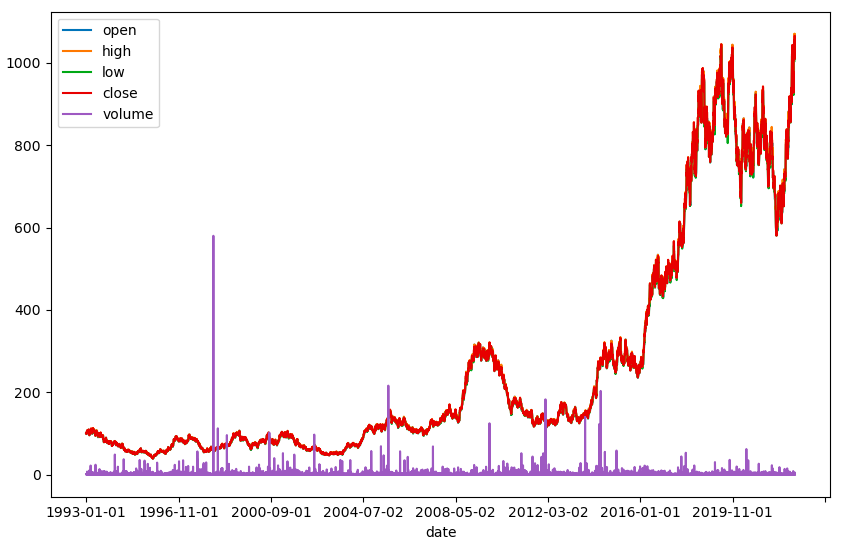
The asset path and volume behaviour (with a much reduced volume multiple) can clearly be seen.
Next Steps
While the combination of the Geometric Brownian Motion SDE and Pareto distribution is a sufficient model to produce asset path data it lacks sophistication compared to real equities data. In particular it is unable to account for mean reversion, stochastic volatility, autocorrelated volumes/prices and other more complex time series behaviours. In future articles the above class will be modified and extended to handle additional time series models.
In addition it will eventually be shown how to execute such a tool on the Raspberry Pi cluster that has been recently been described, in order to create a significant synthetic data library that can be used for backtest model development purposes.
Full Code
# gbm.py

import os
import random
import string

import click
import numpy as np
import pandas as pd


class GeometricBrownianMotionAssetSimulator:
    """
    This callable class will generate a daily
    open-high-low-close-volume (OHLCV) based DataFrame to simulate
    asset pricing paths with Geometric Brownian Motion for pricing
    and a Pareto distribution for volume.

    It will output the results to a CSV with a randomly generated
    ticker smbol.

    For now the tool is hardcoded to generate business day daily
    data between two dates, inclusive.

    Note that the pricing and volume data is completely uncorrelated,
    which is not likely to be the case in real asset paths.

    Parameters
    ----------
    start_date : `str`
        The starting date in YYYY-MM-DD format.
    end_date : `str`
        The ending date in YYYY-MM-DD format.
    output_dir : `str`
        The full path to the output directory for the CSV.
    symbol_length : `int`
        The length of the ticker symbol to use.
    init_price : `float`
        The initial price of the asset.
    mu : `float`
        The mean 'drift' of the asset.
    sigma : `float`
        The 'volatility' of the asset.
    pareto_shape : `float`
        The parameter used to govern the Pareto distribution
        shape for the generation of volume data.
    """

    def __init__(
        self,
        start_date,
        end_date,
        output_dir,
        symbol_length,
        init_price,
        mu,
        sigma,
        pareto_shape
    ):
        self.start_date = start_date
        self.end_date = end_date
        self.output_dir = output_dir
        self.symbol_length = symbol_length
        self.init_price = init_price
        self.mu = mu
        self.sigma = sigma
        self.pareto_shape = pareto_shape

    def _generate_random_symbol(self):
        """
        Generates a random ticker symbol string composed of
        uppercase ASCII characters to use in the CSV output filename.

        Returns
        -------
        `str`
            The random ticker string composed of uppercase letters.
        """
        return ''.join(
            random.choices(
                string.ascii_uppercase,
                k=self.symbol_length
            )
        )

    def _create_empty_frame(self):
        """
        Creates the empty Pandas DataFrame with a date column using
        business days between two dates. Each of the price/volume
        columns are set to zero.

        Returns
        -------
        `pd.DataFrame`
            The empty OHLCV DataFrame for subsequent population.
        """
        date_range = pd.date_range(
            self.start_date,
            self.end_date,
            freq='B'
        )

        zeros = pd.Series(np.zeros(len(date_range)))

        return pd.DataFrame(
            {
                'date': date_range,
                'open': zeros,
                'high': zeros,
                'low': zeros,
                'close': zeros,
                'volume': zeros
            }
        )[['date', 'open', 'high', 'low', 'close', 'volume']]

    def _create_geometric_brownian_motion(self, data):
        """
        Calculates an asset price path using the analytical solution
        to the Geometric Brownian Motion stochastic differential
        equation (SDE).

        This divides the usual timestep by four so that the pricing
        series is four times as long, to account for the need to have
        an open, high, low and close price for each day. These prices
        are subsequently correctly bounded in a further method.

        Parameters
        ----------
        data : `pd.DataFrame`
            The DataFrame needed to calculate length of the time series.

        Returns
        -------
        `np.ndarray`
            The asset price path (four times as long to include OHLC).
        """
        n = len(data)
        T = n / 252.0  # Business days in a year
        dt = T / (4.0 * n)  # 4.0 is needed as four prices per day are required

        # Vectorised implementation of asset path generation
        # including four prices per day, used to create OHLC
        asset_path = np.exp(
            (self.mu - self.sigma**2 / 2) * dt +
            self.sigma * np.random.normal(0, np.sqrt(dt), size=(4 * n))
        )

        return self.init_price * asset_path.cumprod()

    def _append_path_to_data(self, data, path):
        """
        Correctly accounts for the max/min calculations required
        to generate a correct high and low price for a particular
        day's pricing.

        The open price takes every fourth value, while the close
        price takes every fourth value offset by 3 (last value in
        every block of four).

        The high and low prices are calculated by taking the max
        (resp. min) of all four prices within a day and then
        adjusting these values as necessary.

        This is all carried out in place so the frame is not returned
        via the method.

        Parameters
        ----------
        data : `pd.DataFrame`
            The price/volume DataFrame to modify in place.
        path : `np.ndarray`
            The original NumPy array of the asset price path.
        """
        data['open'] = path[0::4]
        data['close'] = path[3::4]

        data['high'] = np.maximum(
            np.maximum(path[0::4], path[1::4]),
            np.maximum(path[2::4], path[3::4])
        )

        data['low'] = np.minimum(
            np.minimum(path[0::4], path[1::4]),
            np.minimum(path[2::4], path[3::4])
        )

    def _append_volume_to_data(self, data):
        """
        Utilises a Pareto distribution to simulate non-negative
        volume data. Note that this is not correlated to the
        underlying asset price, as would likely be the case for
        real data, but it is a reasonably effective approximation.

        Parameters
        ----------
        data : `pd.DataFrame`
            The DataFrame to append volume data to, in place.
        """
        data['volume'] = np.array(
            list(
                map(
                    int,
                    np.random.pareto(
                        self.pareto_shape,
                        size=len(data)
                    ) * 1000000.0
                )
            )
        )

    def _output_frame_to_dir(self, symbol, data):
        """
        Output the fully-populated DataFrame to disk into the
        desired output directory, ensuring to trim all pricing
        values to two decimal places.

        Parameters
        ----------
        symbol : `str`
            The ticker symbol to name the file with.
        data : `pd.DataFrame`
            The DataFrame containing the generated OHLCV data.
        """
        output_file = os.path.join(self.output_dir, '%s.csv' % symbol)
        data.to_csv(output_file, index=False, float_format='%.2f')

    def __call__(self):
        """
        The entrypoint for generating the asset OHLCV frame. Firstly this
        generates a symbol and an empty frame. It then populates this
        frame with some simulated GBM data. The asset volume is then appended
        to this data and finally it is saved to disk as a CSV.
        """
        symbol = self._generate_random_symbol()
        data = self._create_empty_frame()
        path = self._create_geometric_brownian_motion(data)
        self._append_path_to_data(data, path)
        self._append_volume_to_data(data)
        self._output_frame_to_dir(symbol, data)


@click.command()
@click.option('--num-assets', 'num_assets', default='1', help='Number of separate assets to generate files for')
@click.option('--random-seed', 'random_seed', default='42', help='Random seed to set for both Python and NumPy for reproducibility')
@click.option('--start-date', 'start_date', default=None, help='The starting date for generating the synthetic data in YYYY-MM-DD format')
@click.option('--end-date', 'end_date', default=None, help='The starting date for generating the synthetic data in YYYY-MM-DD format')
@click.option('--output-dir', 'output_dir', default=None, help='The location to output the synthetic data CSV file to')
@click.option('--symbol-length', 'symbol_length', default='5', help='The length of the asset symbol using uppercase ASCII characters')
@click.option('--init-price', 'init_price', default='100.0', help='The initial stock price to use')
@click.option('--mu', 'mu', default='0.1', help='The drift parameter, \mu for the GBM SDE')
@click.option('--sigma', 'sigma', default='0.3', help='The volatility parameter, \sigma for the GBM SDE')
@click.option('--pareto-shape', 'pareto_shape', default='1.5', help='The shape of the Pareto distribution simulating the trading volume')
def cli(num_assets, random_seed, start_date, end_date, output_dir, symbol_length, init_price, mu, sigma, pareto_shape):
    num_assets = int(num_assets)
    random_seed = int(random_seed)
    symbol_length = int(symbol_length)
    init_price = float(init_price)
    mu = float(mu)
    sigma = float(sigma)
    pareto_shape = float(pareto_shape)

    # Need to seed both Python and NumPy separately
    random.seed(random_seed)
    np.random.seed(seed=random_seed)

    gbmas = GeometricBrownianMotionAssetSimulator(
        start_date,
        end_date,
        output_dir,
        symbol_length,
        init_price,
        mu,
        sigma,
        pareto_shape
    )

    # Create num_assets files by repeatedly calling
    # the instantiated class
    for i in range(num_assets):
        print('Generating asset path %d of %d...' % (i+1, num_assets))
        gbmas()


if __name__ == "__main__":
    cli()


