In last week's article we looked at Time Series Analysis as a means of helping us create trading strategies. In this article we are going to look at one of the most important aspects of time series, namely serial correlation (also known as autocorrelation).

Before we dive into the definition of serial correlation we will discuss the broad purpose of time series modelling and why we're interested in serial correlation.

When we are given one or more financial time series we are primarily interested in forecasting or simulating data. It is relatively straightforward to identify deterministic trends as well as seasonal variation and decompose a series into these components. However, once such a time series has been decomposed we are left with a random component.

Sometimes such a time series can be well modelled by independent random variables. However, there are many situations, particularly in finance, where consecutive elements of this random component time series will possess correlation. That is, the behaviour of sequential points in the remaining series affect each other in a dependent manner. One major example occurs in mean-reverting pairs trading. Mean-reversion shows up as correlation between sequential variables in time series.

Our task as quantitative modellers is to try and identify the structure of these correlations, as they will allow us to markedly improve our forecasts and thus the potential profitability of a strategy. In addition identifying the correlation structure will improve the realism of any simulated time series based on the model. This is extremely useful for improving the effectiveness of risk management components of the strategy implementation.

When sequential observations of a time series are correlated in the manner described above we say that serial correlation (or autocorrelation) exists in the time series.

Now that we have outlined the usefulness of studying serial correlation we need to define it in a rigourous mathematical manner. Before we can do that we must build on simpler concepts, including expectation and variance.

Expectation, Variance and Covariance

Many of these definitions will be familiar to most QuantStart readers, but I am going to outline them specifically for purposes of consistent notation.

The first definition is that of the expected value or expectation:

Now that we have the definition of expectation we can define the variance, which characterises the "spread" of a random variable:

Notice that the variance is always non-negative. This allows us to define the standard deviation:

Now that we've outlined these elementary statistical definitions we can generalise the variance to the concept of covariance between two random variables. Covariance tells us how linearly related these two variables are:

Covariance tells us how two variables move together.

However since we are in a statistical situation we do not have access to the population means $\mu_x$ and $\mu_y$. Instead we must estimate the covariance from a sample. For this we use the respective sample means $\bar{x}$ and $\bar{y}$.

If we consider a set of $n$ pairs of elements of random variables from $x$ and $y$, given by $(x_i, y_i)$, the sample covariance, $\text{Cov}(x,y)$ (also sometimes denoted by $q(x,y)$) is given by:

Note: Some of you may be wondering why we divide by $n-1$ in the denominator, rather than $n$. This is a valid question! The reason we choose $n-1$ is that it makes $\text{Cov}(x,y)$ an unbiased estimator.

Example: Sample Covariance in R

This is actually our first usage of R on QuantStart. I am not going to discuss the installation procedure of R here, but I will do so in later articles. Thankfully it is much more straightforward than installing Python! Assuming you have R installed you can open up the R terminal.

In the following commands we are going to simulate two vectors of length 100, each with a linearly increasing sequence of integers with some normally distributed noise added. Thus we are constructing linearly associated variables by design.

We will firstly construct a scatter plot and then calculate the sample covariance using the cor function. In order to ensure you see exactly the same data as I do, we will set a random seed of 1 and 2 respectively for each variable:

> set.seed(1)
> x <- seq(1,100) + 20.0*rnorm(1:100)
> set.seed(2)
> y <- seq(1,100) + 20.0*rnorm(1:100)
> plot(x,y)

The plot is as follows:

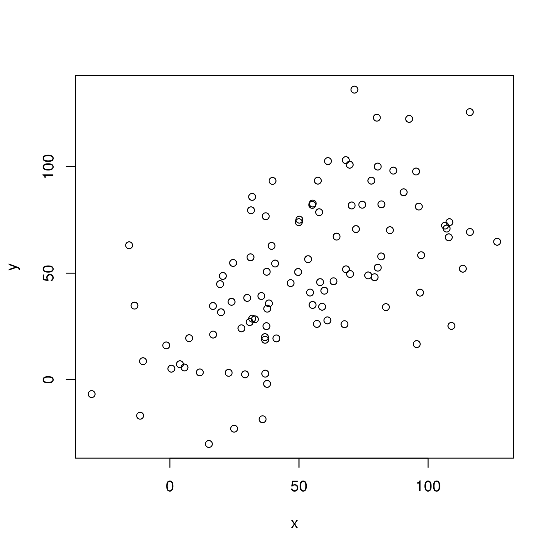Scatter plot of two linearly increasing variables with normally distributed noise

There is a relatively clear association between the two variables. We can now calculate the sample covariance:

> cov(x,y)

681.6859

The sample covariance is given as 681.6859.

One drawback of using the covariance to estimate linear association between two random variables is that it is a dimensional measure. That is, it isn't normalised by the spread of the data and thus it is hard to draw comparisons between datasets with large differences in spread. This motivates another concept, namely correlation.

Correlation

Correlation is a dimensionless measure of how two variables vary together, or "co-vary". In essence, it is the covariance of two random variables normalised by their respective spreads. The (population) correlation between two variables is often denoted by $\rho(x,y)$:

The denominator product of the two spreads will constrain the correlation to lie within the interval $[-1,1]$:

• A correlation of $\rho(x,y) = +1$ indicates exact positive linear association
• A correlation of $\rho(x,y) = 0$ indicates no linear association at all
• A correlation of $\rho(x,y) = -1$ indicates exact negative linear association

As with the covariance, we can define the sample correlation, $\text{Cor}(x,y)$:

Where $\text{Cov}(x,y)$ is the sample covariance of $x$ and $y$, while $\text{sd}(x)$ is the sample standard deviation of $x$.

Example: Sample Correlation in R

We will use the same $x$ and $y$ vectors of the previous example. The following R code will calculate the sample correlation:

> cor(x,y)

0.5796604

The sample correlation is given as 0.5796604 showing a reasonably strong positive linear association between the two vectors, as expected.

Stationarity in Time Series

Now that we outlined the general definitions of expectation, variance, standard deviation, covariance and correlation we are in a position to discuss how they apply to time series data.

Firstly, we will discuss a concept known as stationarity. This is an extremely important aspect of time series and much of the analysis carried out on financial time series data will concern stationarity. Once we have discussed stationarity we are in a position to talk about serial correlation and construct some correlogram plots.

We will begin by trying to apply the above definitions to time series data, starting with the mean/expectation:

There are two important points to note about this definition:

• $\mu = \mu(t)$, i.e. the mean (in general) is a function of time.
• This expectation is taken across the ensemble population of all the possible time series that could have been generated under the time series model. In particular, it is NOT the expression $(x_1 + x_2 + ... + x_k)/k$ (more on this below).

This definition is useful when we are able to generate many realisations of a time series model. However in real life this is usually not the case! We are "stuck" with only one past history and as such we will often only have access to a single historical time series for a particular asset or situation.

So how do we proceed if we wish to estimate the mean, given that we don't have access to these hypothetical realisations from the ensemble? Well, there are two options:

• Simply estimate the mean at each point using the observed value.
• Decompose the time series to remove any deterministic trends or seasonality effects, giving a residual series. Once we have this series we can make the assumption that the residual series is stationary in the mean, i.e. that $\mu(t) = \mu$, a fixed value independent of time. It then becomes possible to estimate this constant population mean using the sample mean $\bar{x} = \sum^{n}_{t=1} \frac{x_t}{n}$.

Now that we've seen how we can discuss expectation values we can use this to flesh out the definition of variance. Once again we make the simplifying assumption that the time series under consideration is stationary in the mean. With that assumption we can define the variance:

This is a straightforward extension of the variance defined above for random variables, except that $\sigma^2 (t)$ is a function of time. Importantly, you can see how the definition strongly relies on the fact that the time series is stationary in the mean (i.e. that $\mu$ is not time-dependent).

You might notice that this definition leads to a tricky situation. If the variance itself varies with time how are we supposed to estimate it from a single time series? As before, the presence of $E(..)$ requires an ensemble of time series and yet we will often only have one!

Once again, we simplify the situation by making an assumption. In particular, and as with the mean, we assume a constant population variance, denoted $\sigma^2$, which is not a function of time. Once we have made this assumption we are in a position to estimate its value using the sample variance definition above:

Note for this to work we need to be able to estimate the sample mean, $\bar{x}$. In addition, as with the sample covariance defined above, we must use $n-1$ in the denominator in order to make the sample variance an unbiased estimator.

This is where we need to be careful! With time series we are in a situation where sequential observations may be correlated. This will have the effect of biasing the estimator, i.e. over- or under-estimating the true population variance.

This will be particularly problematic in time series where we are short on data and thus only have a small number of observations. In a high correlation series, such observations will be close to each other and thus will lead to bias.

In practice, and particularly in high-frequency finance, we are often in a situation of having a substantial number of observations. The drawback is that we often cannot assume that financial series are truly stationary in the mean or stationary in the variance.

As we progress with this article series and develop more sophisticated models, we will address these issues in order to improve our forecasts and simulations.

We are now in a position to apply our time series definitions of mean and variance to that of serial correlation.

Serial Correlation

The essence of serial correlation is that we wish to see how sequential observations in a time series affect each other. If we can find structure in these observations then it will likely help us improve our forecasts and simulation accuracy. This will lead to greater profitability in our trading strategies or better risk management approaches.

Firstly, another definition. If we assume, as above, that we have a time series that is stationary in the mean and stationary in the variance then we can talk about second order stationarity:

Finally, we are in a position to define serial covariance and serial correlation!

The autocovariance $C_k$ is not a function of time. This is because it involves an expectation $E(..)$, which, as before, is taken across the population ensemble of possible time series realisations. This means it is the same for all times $t$.

As before this motivates the definition of serial correlation or autocorrelation, simply by dividing through by the square of the spread of the series. This is possible because the time series is stationary in the variance and thus $\sigma^2 (t) = \sigma^2$:

Note that $\rho_0 = \frac{C_0}{\sigma^2} = \frac{E[(x_t - \mu)^2]}{\sigma^2} = \frac{\sigma^2}{\sigma^2} = 1$. That is, the first lag of $k=0$ will always give a value of unity.

As with the above definitions of covariance and correlation, we can define the sample autocovariance and sample autocorrelation. In particular, we denote the sample autocovariance with a lower-case $c$ to differentiate between the population value given by an upper-case $C$.

The sample autocovariance function $c_k$ is given by:

The sample autocorrelation function $r_k$ is given by:

Now that we have defined the sample autocorrelation function we are in a position to define and plot the correlogram, an essential tool in time series analysis.

The Correlogram

A correlogram is simply a plot of the autocorrelation function for sequential values of lag $k=0,1,...,n$. It allows us to see the correlation structure in each lag.

The main usage of correlograms is to detect any autocorrelation subsequent to the removal of any deterministic trends or seasonality effects.

If we have fitted a time series model then the correlogram helps us justify that this model is well fitted or whether we need to further refine it to remove any additional autocorrelation.

Here is an example correlogram, plotted in R using the acf function, for a sequence of normally distributed random variables. The full R code is as follows:

> set.seed(1)
> w <- rnorm(100)
> acf(w)

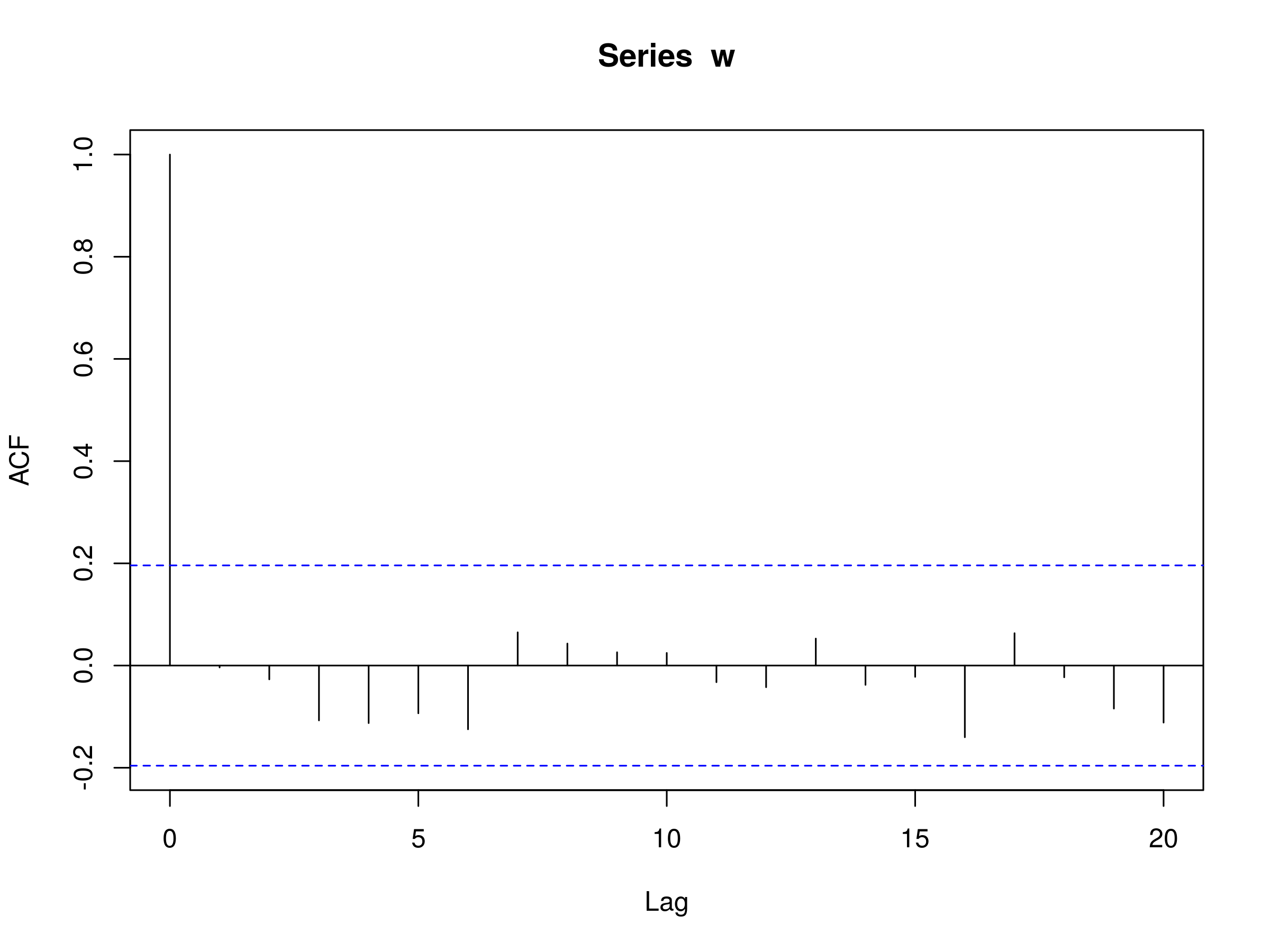Correlogram plotted in R of a sequence of normally distributed random variables

There are a few notable features of the correlogram plot in R:

• Firstly, since the sample correlation of lag $k=0$ is given by $r_0 = \frac{c_0}{c_0} = 1$ we will always have a line of height equal to unity at lag $k=0$ on the plot. In fact, this provides us with a reference point upon which to judge the remaining autocorrelations at subsequent lags. Note also that the y-axis ACF is dimensionless, since correlation is itself dimensionless.
• The dotted blue lines represent boundaries upon which if values fall outside of these, we have evidence against the null hypothesis that our correlation at lag $k$, $r_k$, is equal to zero at the 5% level. However we must take care because we should expect 5% of these lags to exceed these values anyway! Further we are displaying correlated values and hence if one lag falls outside of these boundaries then proximate sequential values are more likely to do so as well. In practice we are looking for lags that may have some underlying reason for exceeding the 5% level. For instance, in a commodity time series we may be seeing unanticipated seasonality effects at certain lags (possibly monthly, quarterly or yearly intervals).

Here are a couple of examples of correlograms for sequences of data.

Example 1 - Fixed Linear Trend

The following R code generates a sequence of integers from 1 to 100 and then plots the autocorrelation:

> w <- seq(1, 100)
> acf(w)

The plot is as follows:

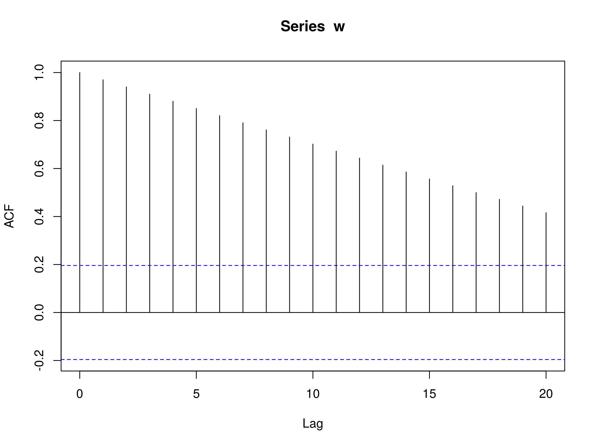Correlogram plotted in R of a sequence of integers from 1 to 100

Notice that the ACF plot decreases in an almost linear fashion as the lags increase. Hence a correlogram of this type is clear indication of a trend.

Example 2 - Repeated Sequence

The following R code generates a repeated sequence of numbers with period $p=10$ and then plots the autocorrelation:

> w <- rep(1:10, 10)
> acf(w)

The plot is as follows:

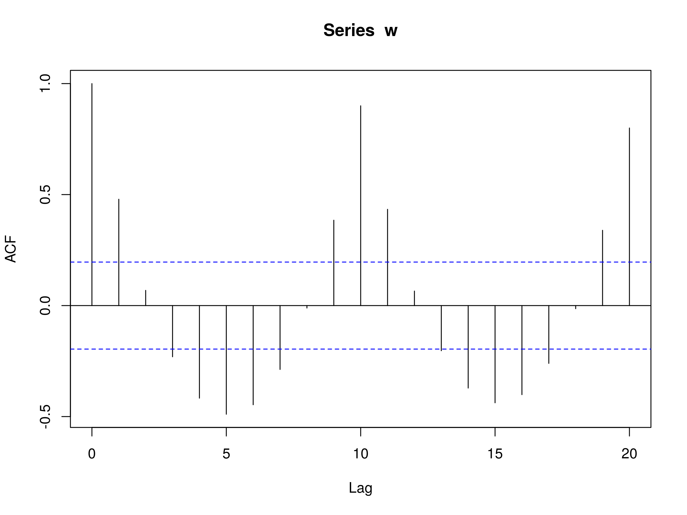Correlogram plotted in R of a sequence of integers from 1 to 10, repeated 10 times

We can see that at lag 10 and 20 there are significant peaks. This makes sense, since the sequences are repeating with a period of 10. Interestingly, note that there is a negative correlation at lags 5 and 15 of exactly -0.5. This is very characteristic of seasonal time series and behaviour of this sort in a correlogram is usually indicative that seasonality/periodic effects have not fully been accounted for in a model.

Next Steps

Now that we've discussed autocorrelation and correlograms in some depth, in future articles we will be moving on to linear models and begin the process of forecasting.

While linear models are far from the state of the art in time series analysis, we need to develop the theory on simpler cases before we can apply it to the more interesting non-linear models that are in use today.