In the previous article in this series we installed and configured SLURM to enable us to parellelise work loads. In this article we will be using SLURM to install QSTrader on all our secondary nodes. This will enable us to run multiple parameter sweeps for backtests of single or multiple strategies in parallel. By the end of this article we will have QSTrader installed and running the example sixty-forty strategy.
Installing the Packages
The first task is to check our Python installation and install the necessary system packages. In part 2 of this article series we installed Ubuntu 22.04 onto our Raspberry Pis. Ubuntu 22.04 comes with Python 3.8 preinstalled at the system level. We first ssh into the primary node (see part 2 of this series for details on SSH and finding the IP address with NMAP).
ssh ubuntu@YOUR-IP-ADDRESS
Where YOUR-IP-ADDRESS should be replaced with the IP address of the primary Raspberry Pi. You will be asked to enter a password. This will be either the default or your chosen password.
As we have SLURM up and running we are able to use the primary node to run commands simultaneously on all the secondary nodes. First we will check to see whether Python is installed on all the secondary nodes. In the primary node type the following:
srun --nodes=3 python3 --version
srun will run a command on as many nodes/cores as you require. In this case we run the command python3 --version on all three of our secondary nodes. If you are using a different number of nodes you simply need to replace the '3' with the correct number of nodes. The command should return something similar to that shown below.
Python 3.8.10
Python 3.8.10
Python 3.8.10
If Python is not installed you will see the following error. If this occurs you can simply add Python3 as an additional package to install in the next step.
srun: error: node04: task 2: Exited with exit code 2
slurmstepd-node04: error: execve(): python3: No such file or directory
slurmstepd-node03: error: execve(): python3: No such file or directory
slurmstepd-node02: error: execve(): python3: No such file or directory
srun: error: node03: task 1: Exited with exit code 2
srun: error: node02: task 0: Exited with exit code 2
We will now install the necessary packages onto all the secondary nodes using the srun command. These include:
pip3the python package managerpython3-venvfor creating virtual environmentspython3-devfor creating the header files needed to build python extensionsbuild-essentialneccessary for compiling softwarevima text editor neccessary for creating SLURM batch scripts, this can be replaced with your chosen text editor- If you recieved an error when testing the Python installation you will also need to add
python3
These will need to be installed as root.
sudo su -
srun --nodelist=YOUR_NODE_NAME[02,03,04] apt install build-essential vim python3-dev python3-pip python3-venv -y
Notice here that we are using the --nodelist flag with srun. This ensures that the commands will be run on each of our nodes, rather than on the first available nodes. When using srun this behaviour is usually default and you can use the --nodes=num_of_nodes instead. However, when using sbatch if your system has been configured to use the consumable resources plugin (as we did in part 3) the nodes will not be assigned exclusively. They will be assigned based on availability and will not necessarily be every node in your system. The --nodelist parameter forces the system to run the code on each node in the list. Remember to replace YOUR_NODE_NAME with the name you gave to your nodes in part 3 of this series.
Creating the Virtual Environment and Installing QSTrader
Once the packages have finished installing you can exit root by typing exit. We can create a virtual environment called 'backtest' on all our secondary nodes where we will install QSTrader.
srun --nodelist=YOUR_NODE_NAME[02,03,04] python3 -m venv backtest
Now if you ssh into each of you Raspberry Pis you will see a new folder backtest inside the home directory. Within this folder you will see a bin directry which contains a pip3 file and a symlink to python3. We will be using both of these to access the virtual environment, first to install QSTrader and then to run QSTrader in our batch file.
To complete the install we can now run the following command using srun. This will use pip3 located inside the virtual environment to install QSTrader into that environment. Remember to repalce your paths and names!
srun --nodelist=YOUR_NODE_NAME[02,03,04] /PATH_TO_YOUR_VENV/backtest/bin/pip3 install qstrader
To check your installation it is best to SSH into each node and run pip freeze within your virtual environment.
Testing QSTrader
In order to test the QSTrader is working we will now run the example 60-40 strategy on all the secondary nodes. This will repeat the same job on all of the nodes allowing us to check that our installation is working correctly. In order to run the example we will need to download the CSV files for the AGG and SPY ETFs. Then we will make some changes to the sixty_forty.py script to allow the output to be saved as JSON file, rather than directly plotting the tearsheet. We will then create a batch file to run the job. All these three files will need to be created or added to the /sharedfs/ shared storage that was configured in part two of this series.
We begin by downloading the CSV files SPY and AGG from yahoo finance. Make sure you download the full history for each. More information on the strategy is available here. Once you have the CSV files we will copy them into the shared storage on the primary node using scp. Remember to replace YOUR_IP_ADDRESS with the ip address of your primary node, you will also need the password.
scp AGG.csv SPY.csv ubuntu@YOUR_IP_ADDRESS:/sharedfs/
We can now create sixty_forty.py in the sharedfs drive and edit it in your chosen text editor. We are using vim. Using ssh, on the primary node run the following commands.
cd /sharedfs/
touch sixty_forty.py
vim sixty_forty.py
The code for the sixty-forty strategy can be copied from the example in the github repository and pasted directly into this file. Once you have pasted the original code we will need to make a few adjustments so that the code can be run in a headless, parallel environment. First we need to remove the function that plots the backtest statistics to a tearsheet and replace it with a function that allows the statistics to be saved to a JSON file. This will allow us to store rather than visualise the backtest information. As we are running the code across multiple nodes we will also make an adjustment to the output file name so that we get a file from each of the nodes, rather that one which has been overwritten.
First let's adjust the import statements. We add the standard library socket. This allows us to get the hostname of each node and append it to the output JSON file. This way we can be sure that QSTrader has been run on each of the nodes. Next we remove the tearsheet import and replace it with an import statement from the JSONStatistics class.
import os
# NEW
import socket

import pandas as pd
import pytz

from qstrader.alpha_model.fixed_signals import FixedSignalsAlphaModel
from qstrader.asset.equity import Equity
from qstrader.asset.universe.static import StaticUniverse
from qstrader.data.backtest_data_handler import BacktestDataHandler
from qstrader.data.daily_bar_csv import CSVDailyBarDataSource
# NEW
from qstrader.statistics.json_statistics import JSONStatistics
# Line below is removed
#from qstrader.statistics.tearsheet import TearsheetStatistics
from qstrader.trading.backtest import BacktestTradingSession
Next we need to edit the dates on the script to be the same as the period covering the data. Inside the main statement you will need to modify the end_dt variable to the last date available from the data you have downloaded. In our case we downloaded data up to the October 3rd 2022 so we will make the following modifcations.
if __name__ == "__main__":
    start_dt = pd.Timestamp('2003-09-30 14:30:00', tz=pytz.UTC)
    end_dt = pd.Timestamp('2022-10-03 23:59:00', tz=pytz.UTC)
Now we need to remove the invocation of the TearsheetStatistic class and replace it with a call to the JSONStatistics class we have just imported. The JSONStatistics class requires a Pandas DataFrame containing the datetime indexed equity curve. This is contained within the strategy_backtest variable which calls the BacktestTradingSession class. It can be obtained by calling the get_equity_curve() method.
The first keyword argument we pass to JSONStatistics is equity_curve=strategy_backtest.get_equity_curve(). The next keyword argument gives our strategy an optional name strategy_name="sixty_forty". We also need to name our output file, here we will use the socket library to get the hostname from our nodes output_filename="sixty_forty_test_%s".json" % socket.gethostname(). The final keyword deals with target allocations. For some strategies QSTrader requires target allocations to enable portfolio rebalancing. This is not necessary for the sixty_forty strategy so we can instead pass an empty Pandas DataFrame. The final keyword argument we need to pass to our invocation of the JSONStatistics class is target_allocations=pd.DataFrame(). The code should look as below.
# NEW
    # Code to enable JSON Output
    backtest_statistics = JSONStatistics(
        equity_curve = strategy_backtest.get_equity_curve(),
        strategy_name = "sixty_forty",
        output_filename = "sixty_forty_test_%s.json" % socket.gethostname(),
        target_allocations = pd.DataFrame()
    )
    backtest_statistics.to_file()

"""
    The following code needs to be removed
    # Performance Output
    tearsheet = TearsheetStatistics(
        strategy_equity=strategy_backtest.get_equity_curve(),
        benchmark_equity=benchmark_backtest.get_equity_curve(),
        title='60/40 US Equities/Bonds'
    )
    tearsheet.plot_results()
"""
The complete code is given below:
import os
import socket

import pandas as pd
import pytz

from qstrader.alpha_model.fixed_signals import FixedSignalsAlphaModel
from qstrader.asset.equity import Equity
from qstrader.asset.universe.static import StaticUniverse
from qstrader.data.backtest_data_handler import BacktestDataHandler
from qstrader.data.daily_bar_csv import CSVDailyBarDataSource
from qstrader.statistics.json_statistics import JSONStatistics
from qstrader.trading.backtest import BacktestTradingSession


if __name__ == "__main__":
    start_dt = pd.Timestamp('2003-09-30 14:30:00', tz=pytz.UTC)
    end_dt = pd.Timestamp('2022-10-03 23:59:00', tz=pytz.UTC)

    # Construct the symbols and assets necessary for the backtest
    strategy_symbols = ['SPY', 'AGG']
    strategy_assets = ['EQ:%s' % symbol for symbol in strategy_symbols]
    strategy_universe = StaticUniverse(strategy_assets)

    # To avoid loading all CSV files in the directory, set the
    # data source to load only those provided symbols
    csv_dir = os.environ.get('QSTRADER_CSV_DATA_DIR', '.')
    data_source = CSVDailyBarDataSource(csv_dir, Equity, csv_symbols=strategy_symbols)
    data_handler = BacktestDataHandler(strategy_universe, data_sources=[data_source])

    # Construct an Alpha Model that simply provides
    # static allocations to a universe of assets
    # In this case 60% SPY ETF, 40% AGG ETF,
    # rebalanced at the end of each month
    strategy_alpha_model = FixedSignalsAlphaModel({'EQ:SPY': 0.6, 'EQ:AGG': 0.4})
    strategy_backtest = BacktestTradingSession(
        start_dt,
        end_dt,
        strategy_universe,
        strategy_alpha_model,
        rebalance='end_of_month',
        long_only=True,
        cash_buffer_percentage=0.01,
        data_handler=data_handler
    )
    strategy_backtest.run()

    # Construct benchmark assets (buy & hold SPY)
    benchmark_assets = ['EQ:SPY']
    benchmark_universe = StaticUniverse(benchmark_assets)

    # Construct a benchmark Alpha Model that provides
    # 100% static allocation to the SPY ETF, with no rebalance
    benchmark_alpha_model = FixedSignalsAlphaModel({'EQ:SPY': 1.0})
    benchmark_backtest = BacktestTradingSession(
        start_dt,
        end_dt,
        benchmark_universe,
        benchmark_alpha_model,
        rebalance='buy_and_hold',
        long_only=True,
        cash_buffer_percentage=0.01,
        data_handler=data_handler
    )
    benchmark_backtest.run()

    # JSON Output
    backtest_statistics = JSONStatistics(
        equity_curve = strategy_backtest.get_equity_curve(),
        strategy_name = "sixty_forty",
        output_filename = "sixty_forty_test_%s.json" % socket.gethostname(),
        target_allocations = pd.DataFrame()
    )
    backtest_statistics.to_file()
Once you have modified the file, copied across the CSV files and saved them to the shared storage directory on the master node you should have everything ready to execute QSTrader using SLURM.
Now we will create our first batch file which we will run using the command sbatch. This command is the usual way to run SLURM jobs. It takes a number of configuration flags and a shell script or batch file. The top of the batch file includes a shebang which will tell SLURM what the required resources are to run the job. Inside the primary node create the batch file, we have chosen to name our batch file "sub_test_qstrader.sh" but you can call it anything you wish. Ensure that the file extension is .sh. Open the file in your chosen text editor.
touch sub_test_qstrader.sh
vim sub_test_qstrader.sh
As we are attempting to test QSTrader across all nodes we will use the #SBATCH --nodelist flag to run the commands across a specified list of nodes and we use srun to execute the commands. Add the following lines to the shell script, remembering to replace YOUR_NODE_NAME with the hostname of your nodes and PATH_TO_YOUR_ENV with the path to your virtual environment. If you are unsure how to find this, SSH into one of the Raspberry Pis and activate the virtual environment as normal. Then type echo $VIRTUAL_ENV. This will give you the path.
#!/bin/bash
#SBATCH --job-name="test_qstrader"
#SBATCH -D .
#SBATCH --output=./logs_%j.out
#SBATCH --error=./logs_%j.err
#SBATCH --nodes=3
#SBATCH --ntasks-per-node=1
#SBATCH --nodelist=YOUR_NODE_NAME[02,03,04]

srun /PATH_TO_YOUR_VENV/backtest/bin/python3 sixty_forty.py
Once you have saved the file you can execute the job by typing
sbatch sub_test_qstrader.sh
The #SBATCH flags are almost identical to those used with srun. A full list can be found by typing sbatch --help into the terminal. The difference between the sbatch and srun flags is that the sbatch flag aren't automaticallly relaunched on specified nodes or cores. The job is instead run on the first core of the first node allcoated to it. The shebang at the top of this file tells SLURM how to allocate our job. Let's look at what each flag is doing.
--job-nameNames the job for ease of identification.--chdirThe directory the job will run in. We have set it to the current directory. You could instead add the linecd $SLURM_SUBMIT_DIRto the main body of the shell script.--outputSaves the standard output to a file for debugging. We have created a file "logs_%j.out" in the current directory, where %j is a placeholder for the SLURM job number.--errorSimilar to --output but saves the standard error.--nodesThe number of nodes you wish to use to run the job.--ntasks-per-nodeNumber of tasks to be carried out on each node.--nodelistRequests specific hosts You will need to use the name of your nodes.
The key flag here is the --nodelist. This ensures that all the commands will be run on each node. As we are testing the software we want to make sure that we are performing this action on all the nodes. We will not need to use this parameter in future, it is only necessary here as a test to ensure that we are running QSTrader on all nodes.
While QSTrader is running we will take a look at another SLURM command squeue. This command allows you to view scheduled jobs. The default view displays the following.
squeue
JOBID PARTITION     NAME               USER ST       TIME  NODES NODELIST(REASON)
    57 mycluster qstrader-test    ubuntu  R       0:03      3     node_name[02-04]
The most important parameter here to note is the ST parameter, which stands for STATUS. A status code of R means the job is running. It is possible to have SLURM send an email once the job has completed. For now we will just use squeue to see if the job has completed.
The other useful command to run is sinfo -lNe. This will allow you to see the nodes running, the partition and the number of CPUS in use.
NODELIST   NODES  PARTITION       STATE CPUS    S:C:T MEMORY TMP_DISK WEIGHT AVAIL_FE REASON
node02       1 mycluster*       mixed    4    4:1:1      1        0      1   (null) none
node03       1 mycluster*       mixed    4    4:1:1      1        0      1   (null) none
node04       1 mycluster*       mixed    4    4:1:1      1        0      1   (null) none
Once the backtest has finished you will have a JSON output file for each of your secondary nodes. As this is a test and we have not varied any of the parameters for the backtests each of these files will contain the same information, the results of a backtest of the sixty-forty strategy holding SPY and AGG. Let's have a look at how to access the information and carry out some simple plots to show first the Equity Curve, compare drawdowns and returns and also the Annual Returns Distribution.
Plotting the Backtest Statistics
In order to analyse and plot the information generated we will be using Pandas and Matplotlib. As our Raspberry Pi server is headless we will not be able to visualise any plots on the system. To visualise the plots you will need to create them on a system that has a GUI so that Matplotlib can generate a window to display the image. This can be done by using TearsheetStatistics class to plot the tearsheet. Once you have one of the output files inside your chosen environment for analysis open up a python console and carry out the following imports.
import json
import pandas as pd
import matplotlib.pyplot as plt
We can now access the information in our output file using the json.load() method from the standard library. Remember to replace YOUR_FILE_NAME with the name of the output file from QSTrader that you are using.
bt = json.load(open("YOUR_FILE_NAME.json", 'r'))
Our variable bt is a dictionary of dictionaries that contains the information from the backtest. We can see the information stored by calling bt['strategy'].keys().
>>> bt['strategy'].keys()
dict_keys(['equity_curve', 'returns', 'cum_returns', 'monthly_agg_returns', 'monthly_agg_returns_hc', 'yearly_agg_returns', 'yearly_agg_returns_hc', 'returns_quantiles', 'returns_quantiles_hc', 'drawdowns', 'max_drawdown', 'max_drawdown_duration', 'mean_returns', 'stdev_returns', 'cagr', 'annualised_vol', 'sharpe', 'sortino', 'target_allocations'])
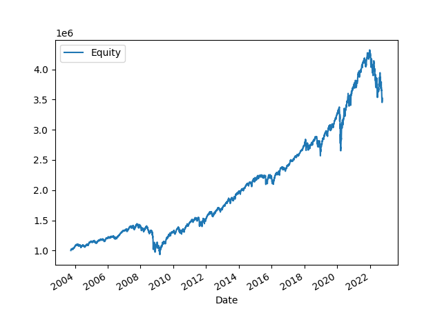
The QSTrader backtest returns a number of useful statistics which we can use to investigate the performance of the strategy. Let's plot the equity curve. First we create a Pandas DataFrame from the equity_curve key. We set the Date as the index.
equity_df = pd.DataFrame(bt['strategy']['equity_curve'], columns=['Date', 'Equity']).set_index('Date')
>>> equity_df
                     Equity
Date
1064880000000  1.000000e+06
1064966400000  1.010972e+06
1065052800000  1.012555e+06
1065139200000  1.015287e+06
1065398400000  1.018659e+06
...                     ...
1664236800000  3.476039e+06
1664323200000  3.538717e+06
1664409600000  3.487817e+06
1664496000000  3.452970e+06
1664755200000  3.518063e+06

[4960 rows x 1 columns]
As you can see the date is stored as the Unix timestamp in milliseconds as an integer. This is the number of milliseconds since January 1st, 1970, 00:00:00. We can convert the date to a human readable format using the following command.
equity_df.index = pd.to_datetime(equity_df.index, unit='ms')
>>> equity_df
                  Equity
Date
2003-09-30  1.000000e+06
2003-10-01  1.010972e+06
2003-10-02  1.012555e+06
2003-10-03  1.015287e+06
2003-10-06  1.018659e+06
...                  ...
2022-09-27  3.476039e+06
2022-09-28  3.538717e+06
2022-09-29  3.487817e+06
2022-09-30  3.452970e+06
2022-10-03  3.518063e+06

[4960 rows x 1 columns]
You can plot and visualise the plot using the following commands.
equity_df.plot()
AxesSubplot:xlabel='Date'
>>> plt.show()
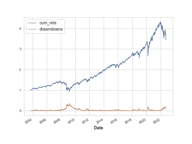
To compare the drawdowns and returns we will need to create two DataFrames and concatenate them together.
cumret_df = pd.DataFrame(bt['strategy']['cum_returns'], columns=['Date', 'cum_rets']).set_index('Date')
>>>drawdown_df = pd.DataFrame(bt['strategy']['drawdowns'], columns=['Date', 'drawndowns']).set_index('Date')
>>>result = pd.concat([eq_df, cumret_df, drawdown_df],axis=1)
We can now plot them as we did before
result.plot()
AxesSubplot:xlabel='Date'
>>> plt.show()
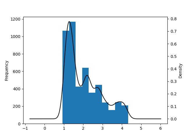
Now let's generate the Annual Returns Distribution. This will require us to create subplots so that we can plot a KDE and a bar chart on the same figure.
fig, ax1 = plt.subplots()
>>> ax1 = result['cum_rets'].plot.hist(bins=10)
>>> ax2 = ax1.twinx()
>>> ax2 = result['cum_rets'].plot.kde(color='black')
>>> plt.show()
If your host environment has a GUI and QSTrader installed you can use the TearsheetStatistics class to plot the tearsheet which is usually generated by QSTrader. This can be done simply by importing the TearsheetStatistics class and passing in the equity_df DataFrame we have just created.
from qstrader.statistics.tearsheet import TearsheetStatistics
>>> tearsheet = TearsheetStatistics(strategy_equity=equity_df, title='60/40 US Equities/Bonds')
>>> tearsheet.plot_results()
Plotting the tearsheet...

This completes the installation and testing of QSTrader on the Raspberry Pi cluster. In the next article in the series we will be running a parameter sweep on a Momentum strategy.


