In this guide I want to introduce you to an extremely powerful machine learning technique known as the Support Vector Machine (SVM). It is one of the best "out of the box" supervised classification techniques. As such, it is an important tool for both the quantitative trading researcher and data scientist.

I feel it is important for a quant researcher or data scientist to be comfortable with both the theoretical aspects and practical usage of the techniques in their toolkit. Hence this article will form the first part in a series of articles that discuss support vector machines. This article specifically will cover the theory of maximal margin classifiers, support vector classifiers and support vector machines. Subsequent articles will make use of the Python scikit-learn library to demonstrate some examples of the aforementioned theoretical techniques on actual data.

Motivation for Support Vector Machines

The problem to be solved in this article is one of supervised binary classification. That is, we wish to categorise new unseen objects into two separate groups based on their properties and a set of known examples, which are already categorised. A good example of such a system is classifying a set of new documents into positive or negative sentiment groups, based on other documents which have already been classified as positive or negative. Similarly, we could classify new emails into spam or non-spam, based on a large corpus of documents that have already been marked as spam or non-spam by humans. SVMs are highly applicable to such situations.

A Support Vector Machine models the situation by creating a feature space, which is a finite-dimensional vector space, each dimension of which represents a "feature" of a particular object. In the context of spam or document classification, each "feature" is the prevalence or importance of a particular word.

The goal of the SVM is to train a model that assigns new unseen objects into a particular category. It achieves this by creating a linear partition of the feature space into two categories. Based on the features in the new unseen objects (e.g. documents/emails), it places an object "above" or "below" the separation plane, leading to a categorisation (e.g. spam or non-spam). This makes it an example of a non-probabilistic linear classifier. It is non-probabilistic, because the features in the new objects fully determine its location in feature space and there is no stochastic element involved.

However, much of the benefit of SVMs comes from the fact that they are not restricted to being linear classifiers. Utilising a technique known as the kernel trick they can become much more flexible by introducing various types of non-linear decision boundaries.

Formally, in mathematical language, SVMs construct linear separating hyperplanes in high-dimensional vector spaces. Data points are viewed as $(\vec{x}, y)$ tuples, $\vec{x} = (x_1, \ldots, x_p)$ where the $x_j$ are the feature values and $y$ is the classification (usually given as $+1$ or $-1$). Optimal classification occurs when such hyperplanes provide maximal distance to the nearest training data points. Intuitively, this makes sense, as if the points are well separated, the classification between two groups is much clearer.

However, if in a feature space some of the sets are not linearly separable (i.e. they overlap!), then it is necessary to perform a mapping of the original feature space to a higher-dimensional space, in which the separation between the groups is clear, or at least clearer. However, this has the consequence of making the separation boundary in the original space potentially non-linear.

In this article we will proceed by considering the advantages and disadvantages of SVMs as a classification technique, then defining the concept of an optimal linear separating hyperplane, which motivates a simple type of linear classifier known as a maximal margin classifier (MMC). We will then show that maximal margin classifiers are not often applicable to many "real world" situations and as such need modification, in the form of a support vector classifier (SVC). We will then relax the restriction of linearity and consider non-linear classifiers, namely support vector machines, which use kernel functions to improve computational efficiency.

Advantages and Disadvantages of SVMs

As a classification technique, the SVM has many advantages, many of which are due to its computational efficiency on large datasets. The Scikit-Learn team have summarised the main advantages and disadvantages here but I have repeated and elaborated on them for completeness:

Advantages

• High-Dimensionality - The SVM is an effective tool in high-dimensional spaces, which is particularly applicable to document classification and sentiment analysis where the dimensionality can be extremely large ($\geq 10^6$).
• Memory Efficiency - Since only a subset of the training points are used in the actual decision process of assigning new members, only these points need to be stored in memory (and calculated upon) when making decisions.
• Versatility - Class separation is often highly non-linear. The ability to apply new kernels allows substantial flexibility for the decision boundaries, leading to greater classification performance.

Disadvantages

• $p > n$ - In situations where the number of features for each object ($p$) exceeds the number of training data samples ($n$), SVMs can perform poorly. This can be seen intuitively, as if the high-dimensional feature space is much larger than the samples, then there are less effective support vectors on which to support the optimal linear hyperplanes, leading to poorer classification performance as new unseen samples are added.
• Non-Probabilistic - Since the classifier works by placing objects above and below a classifying hyperplane, there is no direct probabilistic interpretation for group membership. However, one potential metric to determine "effectiveness" of the classification is how far from the decision boundary the new point is.

Now that we've outlined the advantages and disadvantages, we're going to discuss the geometric objects and mathematical entities that will ultimately allow us to define the SVMs and how they work.

There are some fantastic references (both links and textbooks) that derive much of the mathematical detail of how SVMs work. In the following derivation I didn't want to "reinvent the wheel" too much, especially with regards notation and pedagogy, so I've formulated the following treatment based on the references provided at the end of the article, making strong use of James et al (2013), Hastie et al (2009) and the Wikibooks article on SVMs. I have made changes to the notation where appropriate and have adjusted the narrative to suit individuals interested in quantitative finance.

Linear Separating Hyperplanes

The linear separating hyperplane is the key geometric entity that is at the heart of the SVM. Informally, if we have a high-dimensional feature space, then the linear hyperplane is an object one dimension lower than this space that divides the feature space into two regions.

This linear separating plane need not pass through the origin of our feature space, i.e. it does not need to include the zero vector as an entity within the plane. Such hyperplanes are known as affine.

If we consider a real-valued $p$-dimensional feature space, known mathematically as $\mathbb{R}^p$, then our linear separating hyperplane is an affine $p-1$ dimensional space embedded within it.

For the case of $p=2$ this hyperplane is simply a one-dimensional straight line, which lives in the larger two-dimensional plane, whereas for $p=3$ the hyerplane is a two-dimensional plane that lives in the larger three-dimensional feature space (see Fig 1 and Fig 2):

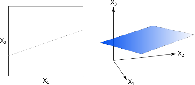
Figs 1 and 2: One- and two-dimensional hyperplanes

If we consider an element of our $p$-dimensional feature space, i.e. $\vec{x}=(x_1,...,x_p) \in \mathbb{R}^p$, then we can mathematically define an affine hyperplane by the following equation:

$b_0 \neq 0$ gives us an affine plane (i.e. it does not pass through the origin). We can use a more succinct notation for this equation by introducing the summation sign:

Notice however that this is nothing more than a multi-dimensional dot product (or, more generally, an inner product), and as such can be written even more succinctly as:

If an element $\vec{x} \in \mathbb{R}^p$ satisfies this relation then it lives on the $p-1$-dimensional hyperplane. This hyperplane splits the $p$-dimensional feature space into two classification regions (see Fig 3):

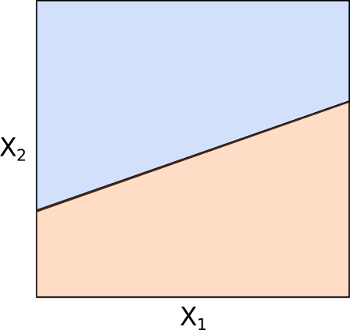
Fig 3: Separation of $p$-dimensional space by a hyperplane

Elements $\vec{x}$ above the plane satisfy:

While those below it satisfy:

The key point here is that it is possible for us to determine which side of the plane any element $\vec{x}$ will fall on by calculating the sign of the expression $\vec{b} \cdot \vec{x} + b_0$. This concept will form the basis of a supervised classification technique.

Classification

Continuing with our example of email spam filtering, we can think of our classification problem (say) as being provided with a thousand emails ($n=1000$), each of which is marked spam ($+1$) or non-spam ($-1$). In addition, each email has an associated set of keywords (i.e. separating the words on spacing) that provide features. Hence if we take the set of all possible keywords from all of the emails (and remove duplicates), we will be left with $p$ keywords in total.

If we translate this into a mathematical problem, the standard setup for a supervised classification procedure is to consider a set of $n$ training observations, $\vec{x}_i$, each of which is a $p$-dimensional vector of features. Each training observation has an associated class label, $y_i \in \{ -1,1 \}$. Hence we can think of $n$ pairs of training observations $(\vec{x}_i, y_i)$ representing the features and class labels (keyword lists and spam/non-spam). In addition to the training observations we can provide test observations, $\vec{x}^{*} = (x^{*}_1, ... , x^{*}_p)$ that are later used to test the performance of the classifiers. In our spam example, these test observations would be new emails that have not yet been seen.

Our goal is to develop a classifier based on provided training observations that will correctly classify subsequent test observations using only their feature values. This translates into being able to classify an email as spam or non-spam solely based on the keywords contained within it.

We will initially suppose that it is possible, via a means yet to be determined, to construct a hyperplane that separates training data perfectly according to their class labels (see Figs 4 and 5). This would mean cleanly separating spam emails from non-spam emails solely by using specific keywords. The following diagram is only showing $p=2$, while for keyword lists we may have $p>10^6$. Hence Figs 4 and 5 are only representative of the problem.

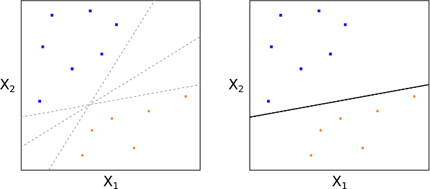
Fig 4: Multiple separating hyperplanes; Fig 5: Perfect separation of class data

This translates into a mathematical separating property of:

and

This basically states that if each training observation is above or below the separating hyperplane, according to the geometric equation which defines the plane, then its associated class label will be $+1$ or $-1$. Thus we have developed a simple classification process. We assign a test observation to a class depending upon which side of the hyperplane it is located on.

This can be formalised by considering the following function $f(\vec{x})$, with a test observation $\vec{x}^{*}=(x^{*}_1,...,x^{*}_p)$:

If $f(\vec{x}^{*}) > 0$ then $y^{*} = +1$, whereas if $f(\vec{x}^{*}) < 0$ then $y^{*} = -1$.

However, this tells us nothing about how we go about finding the $b_j$ components of $\vec{b}$, as well as $b_0$, which are crucial in helping us determine the equation of the hyperplane separating the two regions. The next section discusses an approach for carrying this out, as well as introducing the concept of the maximal margin hyperplane and a classifier built on it, known as the maximal margin classifier.

Deriving the Classifier

At this stage it is worth pointing out that separating hyperplanes are not unique, since it is possible to slightly translate or rotate such a plane without touching any training observations (see Fig 4).

So, not only do we need to know how to construct such a plane, but we also need to determine the most optimal. This motivates the concept of the maximal margin hyperplane (MMH), which is the separating hyperplane that is farthest from any training observations, and is thus "optimal".

How do we find the maximal margin hyperplane? Firstly, we compute the perpendicular distance from each training observation $\vec{x}_i$ for a given separating hyperplane. The smallest perpendicular distance to a training observation from the hyperplane is known as the margin. The MMH is the separating hyperplane where the margin is the largest. This guarantees that it is the farthest minimum distance to a training observation.

The classification procedure is then just simply a case of determining which side a test observation falls on. This can be carried out using the above formula for $f(\vec{x}^{*})$. Such a classifier is known as a maximimal margin classifier (MMC). Note however that finding the particular values that lead to the MMH is purely based on the training observations. That is, we still need to be aware of how the MMC performs on the test observations. We are implicitly making the assumption that a large margin in the training observations will provide a large margin on the test observations, but this may not be the case.

As always, we must be careful to avoid overfitting when the number of feature dimensions is large (e.g. in Natural Language Processing applications such as email spam classification). Overfitting here means that the MMH is a very good fit for the training data but can perform quite poorly when exposed to testing data. I discuss this issue in depth in the article on the bias-variance trade-off.

To reiterate, our goal now becomes finding an algorithm that can produce the $b_j$ values, which will fix the geometry of the hyperplane and hence allow determination of $f(\vec{x}^{*})$ for any test observation.

If we consider Fig 6, we can see that the MMH is the mid-line of the widest "block" that we can insert between the two classes such that they are perfectly separated.

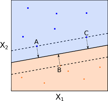
Fig 6: Maximal margin hyperplane with support vectors (A, B and C)

One of the key features of the MMC (and subsequently SVC and SVM) is that the location of the MMH only depends on the support vectors, which are the training observations that lie directly on the margin (but not hyperplane) boundary (see points A, B and C in Fig 6). This means that the location of the MMH is NOT dependent upon any other training observations.

Thus it can be immediately seen that a potential drawback of the MMC is that its MMH (and thus its classification performance) can be extremely sensitive to the support vector locations. However, it is also partially this feature that makes the SVM an attractive computational tool, as we only need to store the support vectors in memory once it has been "trained" (i.e. the $b_j$ values are fixed).

Constructing the Maximal Margin Classifier

I feel it is instructive to fully outline the optimisation problem that needs to be solved in order to create the MMH (and thus the MMC itself). While I will outline the constraints of the optimisation problem, the algorithmic solution to this problem is beyond the scope of the article. Thankfully these optimisation routines are implemented in scikit-learn (actually, via the LIBSVM library). If you wish to read more about the solution to these algorithmic problems, take a look at Hastie et al (2009) and the Scikit-Learn page on Support Vector Machines.

The procedure for determining a maximal margin hyperplane for a maximal margin classifier is as follows. Given $n$ training observations $\vec{x}_1, ..., \vec{x}_n \in \mathbb{R}^p$ and $n$ class labels $y_1,...,y_n \in \{-1,1\}$, the MMH is the solution to the following optimisation procedure:

Maximise $M \in \mathbb{R}$, by varying $b_1, ..., b_p$ such that:

and

Despite the complex looking constraints, they actually state that each observation must be on the correct side of the hyperplane and at least a distance $M$ from it. Since the goal of the procedure is to maximise $M$, this is precisely the condition we need to create the MMC!

Clearly, the case of perfect separability is an ideal one. Most "real world" datasets will not have such perfect separability via a linear hyperplane (see Fig 7). However, if there is no separability then we are unable to construct a MMC by the optimisation procedure above. So, how do we create a form of separating hyperplane?

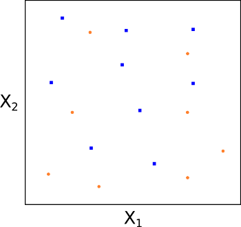
Fig 7: No possibility of a true separating hyperplane

Essentially we have to relax the requirement that a separating hyperplane will perfectly separate every training observation on the correct side of the line (i.e. guarantee that it is associated with its true class label), using what is called a soft margin. This motivates the concept of a support vector classifier (SVC).

Support Vector Classifiers

As we alluded to above, one of the problems with MMC is that they can be extremely sensitive to the addition of new training observations. Consider Figs 8 and 9. In Fig 8 it can be seen that there exists a MMH perfectly separating the two classes. However, in Fig 9 if we add one point to the $+1$ class we see that the location of the MMH changes substantially. Hence in this situation the MMH has clearly been over-fit:

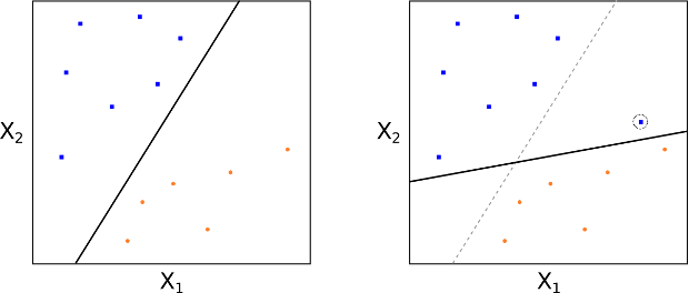
Figs 8 and 9: Addition of a single point dramatically changes the MMH line

As we mentioned above also, we could consider a classifier based on a separating hyperplane that doesn't perfectly separate the two classes, but does have a greater robustness to the addition of new invididual observations and has a better classification on most of the training observations. This comes at the expense of some misclassification of a few training observations.

This is how a support vector classifier or soft margin classifier works. A SVC allows some observations to be on the incorrect side of the margin (or hyperplane), hence it provides a "soft" separation. The following figures 10 and 11 demonstrate observations being on the wrong side of the margin and the wrong side of the hyperplane respectively:

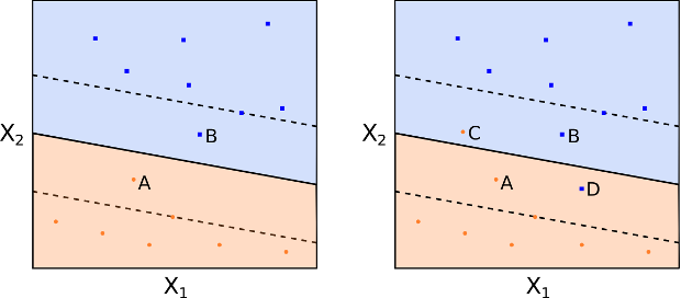
Figs 10 and 11: Observations on the wrong side of the margin and hyperplane, respectively

As before, an observation is classified depending upon which side of the separating hyperplane it lies on, but some points may be misclassified.

It is instructive to see how the optimisation procedure differs from that described above for the MMC. We need to introduce new parameters, namely $n$ $\epsilon_i$ values (known as the slack values) and a parameter $C$, known as the budget. We wish to maximise $M$, across $b_1, ..., b_p,\epsilon_1,..,\epsilon_n$ such that:

and

and

Where $C$, the budget, is a non-negative "tuning" parameter. $M$ still represents the margin and the slack variables $\epsilon_i$ allow the individual observations to be on the wrong side of the margin or hyperplane.

In essence the $\epsilon_i$ tell us where the $i$th observation is located relative to the margin and hyperplane. For $\epsilon_i=0$ it states that the $x_i$ training observation is on the correct side of the margin. For $\epsilon_i>0$ we have that $x_i$ is on the wrong side of the margin, while for $\epsilon_i>1$ we have that $x_i$ is on the wrong side of the hyperplane.

$C$ collectively controls how much the individual $\epsilon_i$ can be modified to violate the margin. $C=0$ implies that $\epsilon_i=0, \forall i$ and thus no violation of the margin is possible, in which case (for separable classes) we have the MMC situation.

For $C>0$ it means that no more than $C$ observations can violate the hyperplane. As $C$ increases the margin will widen. See Fig 12 and 13 for two differing values of $C$:

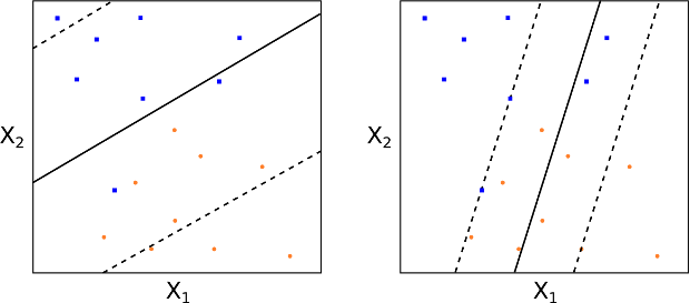
Figs 12 and 13: Different values of the tuning parameter $C$

How do we choose $C$ in practice? Generally this is done via cross-validation. In essence $C$ is the parameter that governs the bias-variance trade-off for the SVC. A small value of $C$ means a low bias, high variance situation. A large value of $C$ means a high bias, low variance situation.

As before, to classify a new test observation $x^{*}$ we simply calculate the sign of $f(\vec{x}^{*})= \vec{b} \cdot \vec{x}^{*} + b_0$.

This is all well and good for classes that are linearly (or nearly linearly) separated. However, what about separation boundaries that are non-linear? How do we deal with those situations? This is where we can extend the concept of support vector classifiers to support vector machines.

Support Vector Machines

The motivation behind the extension of a SVC is to allow non-linear decision boundaries. This is the domain of the Support Vector Machine (SVM). Consider the following Figs 14 and 15. In such a situation a purely linear SVC will have extremely poor performance, simply because the data has no clear linear separation:

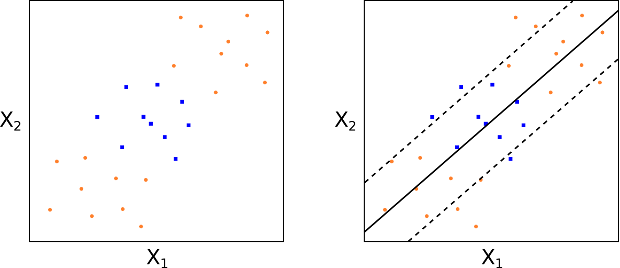
Figs 14 and 15: No clear linear separation between classes and thus poor SVC performance

Hence SVCs can be useless in highly non-linear class boundary problems.

In order to motivate how an SVM works, we can consider a standard "trick" in linear regression, when considering non-linear situations. In particular a set of $p$ features $x_1, ... , x_p$ can be transformed, say, into a set of $2p$ features $x_1, x^2_1, ..., x_p, x^2_p$. This allows us to apply a linear technique to a set of non-linear features.

While the decision boundary is linear in the new $2p$-dimensional feature space it is non-linear in the original $p$-dimensional space. We end up with a decision boundary given by $q(\vec{x})=0$ where $q$ is a quadratic polynomial function of the original features and hence is a non-linear solution.

This is clearly not restricted to quadratic polynomials. Higher dimensional polynomials, interaction terms and other functional forms, could all be considered. Although the drawback is that it dramatically increases the dimension of the feature space to the point that some algorithms can become untractable.

The major advantage of SVMs is that they allow a non-linear enlargening of the feature space, while still retaining a significant computational efficiency, using a process known as the "kernel trick", which will be outlined below shortly.

So what are SVMs? In essence they are an extension of SVCs that results from enlargening the feature space through the use of functions known as kernels. In order to understand kernels, we need to briefly discuss some aspects of the solution to the SVC optimisation problem outlined above.

While calculating the solution to the SVC optimisation problem, the algorithm only needs to make use of inner products between the observations and not the observations themselves. Recall that an inner product is defined for two $p$-dimensional vectors $u,v$ as:

Hence for two observations an inner product is defined as:

While we won't dwell on the details (since they are beyond the scope of this article), it is possible to show that a linear support vector classifier for a particular observation $\vec{x}$ can be represented as a linear combination of inner products:

With $n$ $a_i$ coefficients, one for each of the training observations.

To estimate the $b_0$ and $a_i$ coefficients we only need to calculate ${n \choose 2} = n(n-1)/2$ inner products between all pairs of training observations. In fact, we ONLY need to calculate the inner products for the subset of training observations that represent the support vectors. I will call this subset $\mathscr{S}$. This means that:

This means we can rewrite the representation formula as:

This turns out to be a major advantage for computational efficiency.

This now motivates the extension to SVMs. If we consider the inner product $\langle \vec{x}_i, \vec{x}_k \rangle$ and replace it with a more general inner product "kernel" function $K=K(\vec{x}_i, \vec{x}_k)$, we can modify the SVC representation to use non-linear kernel functions and thus modify how we calculate "similarity" between two observations. For instance, to recover the SVC we just take $K$ to be as follows:

Since this kernel is linear in its features the SVC is known as the linear SVC. We can also consider polynomial kernels, of degree $d$:

This provides a significantly more flexible decision boundary and essentially amounts to fitting a SVC in a higher-dimensional feature space involving $d$-degree polynomials of the features (see Fig 16).

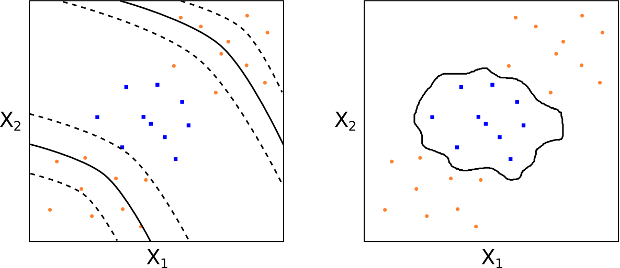
Fig 16: A $d$-degree polynomial kernel; Fig 17: A radial kernel

Hence, the definition of a support vector machine is a support vector classifier with a non-linear kernel function.

We can also consider the popular radial kernel (see Fig 17):

So how do radial kernels work? They are clearly quite different from polynomial kernels. Essentially if our test observation $\vec{x}^{*}$ is far from a training observation $\vec{x}_i$ in standard Euclidean distance then the sum $\sum^{p}_{j=1} (x^{*}_j - x_{ij})^2$ will be large and thus $K(\vec{x}^{*},\vec{x}_i)$ will be very small. Hence this particular training observation $\vec{x}_i$ will have almost no effect on where the test observation $\vec{x}^{*}$ is placed, via $f(\vec{x}^{*})$.

Thus the radial kernel has extremely localised behaviour and only nearby training observations to $\vec{x}^{*}$ will have an impact on its class label.

While this article has been very theoretical, the next article on document classification using Scikit-Learn makes heavy use of SVMs in Python.

Biblographic Notes

Originally, SVMs were invented by Vapnik (1996), while the current standard "soft margin" approach is due to Cortes (1995). My treatment of the material follows, and is strongly influenced by, the excellent statistical machine learning texts of James et al (2013) and Hastie et al (2009).

References

• Vapnik, V. (1996) The Nature of Statistical Learning Theory
• Cortes, C., Vapnik, V. (1995) "Support Vector Networks", Machine Learning 20 (3): 273
• James, G., Witten, D., Hastie, T., Tibshiranie, R. (2013) An Introduction to Statistical Learning
• Hastie, T., Tibshiranie, R., Friedman, J. (2009) The Elements of Statistical Learning
• Wikibooks (2016) Support Vector Machines (Link)
• Scikit-Learn (2016) Support Vector Machines (Link)