In this article I want to discuss one of the most important and tricky issues in machine learning, that of model selection and the bias-variance tradeoff. The latter is one of the most crucial issues in helping us achieve profitable trading strategies based on machine learning techniques.
Model selection refers to our ability to assess performance of differing machine learning models in order to choose the best one.
The bias-variance tradeoff is a particular property of all (supervised) machine learning models, that enforces a tradeoff between how "flexible" the model is and how well it performs on unseen data. The latter is known as a models generalisation performance.
We will begin by understanding why model selection is important and then discuss the bias-variance tradeoff qualitatively. We will wrap up the article by deriving the bias-variance tradeoff mathematically and discuss measures to minimise the problems it introduces.
In this article we are considering supervised regression models. That is, models which are trained on a set of labelled training data and produce a quantitative response. An example of this would be attempting to predict future stock prices based on other factors such as past prices, interest rates or foreign exchange rates.
This is in contrast to a categorical or binary response model as in the case of supervised classification. An example of a classification setting would be attempting to assign a topic to a text document, from a finite set of topics. The bias-variance and model selection situations for classification are extremely similar to the regression setting and simply require modification to handle the differing ways in which errors and performance are measured. We will discuss these modifications in a latter article.
Note: If you wish to learn more about the basic model notation that we will use in this article, it is worth having a read of the article on the basics of statistical machine learning.
Machine Learning Models
As with most of our discussions in machine learning the basic model is given by the following:
\begin{eqnarray} Y = f(X) + \epsilon \end{eqnarray}This states that the response vector, $Y$, is given as a (potentially non-linear) function, $f$, of the predictor vector, $X$, with a set of normally distributed error terms that have mean zero and a standard deviation of one.
What does this mean in practice?
As an example, our vector $X$ could represent a set of lagged financial prices. It could also represent interest rates, derivatives prices, real-estate prices, word-frequencies in a document or any other factor that we consider useful in making a prediction.
The vector $Y$ could be single or multi-valued. In the former case it might simply represent tomorrow's stock price, in the latter case it might represent the next week's daily predicted prices.
$f$ represents our view on the underlying relationship between $Y$ and $X$. This could be linear, in which case we may estimate $f$ via a linear regression model. It may be non-linear, in which case we may estimate $f$ with a Support Vector Machine or a spline-based method, for instance.
The error terms $\epsilon$ represent all of the factors that affect $Y$ that we haven't taken into account with our function $f$. They are essentially the "unknown" components of our prediction model. It is commmon to assume that these are normally distributed with mean zero and a standard deviation of one.
In this article we are going to describe how to measure the performance of an estimate for the (unknown) function $f$. Such an estimate uses "hat" notation. Hence, $\hat{f}$ can be read as "the estimate of $f$".
In addition we will describe the effect on the performance of the model as we make it more flexible. Flexibility describes the ability to increase the degrees of freedom available to the model to "fit" to the training data. We will see that the relationship between flexibility and performance error is non-linear and thus we need to be extremely careful when choosing the "best" model.
Note that there is never a "best" model across the entirety of statistics and machine learning. Different models have varying strengths and weaknesses. One model may work very well on one dataset, but may perform badly on another. The challenge in statistical machine learning is to pick the "best" model for the problem at hand with the data available.
Model Selection
When trying to ascertain which statistical machine learning method is best we need some means of characterising the relative performance between models.
To achieve this we need to compare the known values of the underlying relationship with those that are predicted by an estimated model.
For instance, if we are attempting to predict tomorrow's stock prices, then we wish to evaluate how close our models predictions are to the true value on that particular day.
This motivates the concept of a loss function, which quantitatively compares the difference between the true values with the predicted values.
Let's assume that we have created an estimate $\hat{f}$ of the underlying relationship $f$. $\hat{f}$ might be a linear regression or a Random Forest model, for instance. $\hat{f}$ will have been trained on a particular data set, $\tau$, which contains predictor-response pairs. If there are $N$ such pairs then $\tau$ is given by:
\begin{eqnarray} \tau = \{ (X_1, Y_1), ..., (X_N, Y_N) \} \end{eqnarray}The $X_i$ represent the prediction factors, which could be prior lagged prices for a series or some other factors, as mentioned above. The $Y_i$ could be the predictions for our stock prices in the following period. In this instance, $N$ represents the number of days of data that we have available.
The loss function is denoted by $L(Y, \hat{f}(X))$. Its job is to compare the predictions made by $\hat{f}$ at particular values of $X$ to their true values given by $Y$. A common choice for $L$ is the absolute error:
\begin{eqnarray} L(Y, \hat{f}(X)) = |Y - \hat{f}(X)| \end{eqnarray}Another popular choice is the squared error:
\begin{eqnarray} L(Y, \hat{f}(X)) = (Y - \hat{f}(X))^2 \end{eqnarray}Note that both choices of loss function are non-negative. Hence the "best" loss for a model is zero, that is, there is no difference between the prediction and the true value.
Training Error versus Test Error
Now that we have a loss function we need some way of aggregating the various differences between the true values and the predicted values. One way to do this is to define the Mean Squared Error (MSE), which is simply the average, or expectation value, of the squared loss:
\begin{eqnarray} MSE := \frac{1}{N} \sum^{N}_{i=1} (Y_i - \hat{f}(X_i))^2 \end{eqnarray}The definition simply states that the Mean Squared Error is the average of all of the squared differences between the true values $Y_i$ and the predicted values $\hat{f}(X_i)$. A smaller MSE means that the estimate is more accurate.
It is important to realise that this MSE value is computed using only the training data. That is, it is computed using only the data that the model was fitted on. Hence, it is actually known as the training MSE.
In practice this value is of little interest to us. What we are really concerned about is how well the model can predict values on new unseen data.
For instance, we are not really interested in how well the model can predict past stock prices of the following day, we are only concerned with how it can predict the following days stock prices going forward. This quantification of a models performance is known as its generalisation performance. It is what we are really interested in.
Mathematically, if we have a new prediction value $X_0$ and a true response $Y_0$, then we wish to take the expectation across all such new values to come up with the test MSE:
\begin{eqnarray} \text{Test MSE} := \mathbb{E}\left[ (Y_0 - \hat{f}(X_0))^2 \right] \end{eqnarray}Where the expectation is taken across all new unseen predictor-response pairs $(X_0, Y_0)$.
Our goal is to select the model where the test MSE is lowest across choices of other models.
Unfortunately it is difficult to calculate the test MSE! This is because we are often in a situation where we do not have any test data available.
In general machine learning domains this can be quite common. In quantitative trading we are (usually) in a "data rich" environment and thus we can retain some of our data for training and some for testing. In future articles we will discuss cross-validation, which is one means of utilising subsets of the training data in order to estimate the test MSE.
A pertinent question to ask at this stage is "Why can we not simply use the model with the lowest training MSE?". The simple answer is that we are unable to use this approach because there is no guarantee that the model with the lowest training MSE will also be the model with the lowest test MSE. Why is this so? The answer lies in a particular property of statistical machine learning methods known as the bias-variance tradeoff.
The Bias-Variance Tradeoff
Let's consider a slightly contrived situation where we know the underlying "true" relationship between $Y$ and $X$, which I will state is given by a sinusoidal function, $f = \sin$, such that $Y = f(X) = \sin(X)$. Note that in reality we will not ever know the underlying $f$, which is why we are estimating it in the first place!
For this contrived situation I have created a set of training points, $\tau$, given by $Y_i = \sin(X_i) + \epsilon_i$, where $\epsilon_i$ are draws from a standard normal distribution (mean of zero, standard deviation equal to one). This can be seen in Figure 1. The black curve is the "true" function $f$, restricted to the interval $[0, 2 \pi]$, while the circled points represent the $Y_i$ simulated data values.
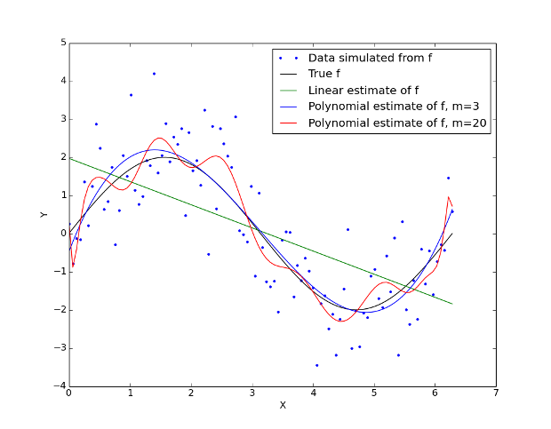 Figure 1 - Various estimates of the underlying sinusoidal model, $f=\sin$.
We can now try to fit a few different models to this training data. The first model, given by the green line, is a linear regression fitted with ordinary least squares estimation. The second model, given by the blue line, is a polynomial model with degree $m=3$. The third model, given by the red curve is a higher degree polynomial with degree $m=20$. Between each of the models I have varied the flexibility, that is, the degrees of freedom (DoF). The linear model is the least flexible with only two DoF. The most flexible model is the polynomial of order $m=20$. It can be seen that the polynomial of order $m=3$ is the apparent closest fit to the underlying sinusoidal relationship.
For each of these models we can calculate the training MSE. It can be seen in Figure 2 that the training MSE (given by the green curve) decreases monotonically as the flexibility of the model increases. This makes sense, since the polynomial fit can become as flexible as we need it to in order to minimise the difference between its values and those of the sinusoidal data.
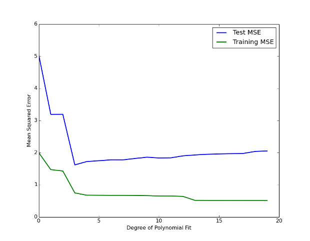 Figure 2 - Training MSE and Test MSE as a function of model flexibility.
However, if we plot the test MSE (given by the blue curve) the situation is vastly different. The test MSE initially decreases as we increase the flexibility of the model but eventually starts to increase again after we introduce a lot of flexibility. Why is this? By allowing the model to be extremely flexible we are letting it fit to "patterns" in the training data.
However, as soon as we introduce new unseen data points in the test set the model cannot generalise well because these "patterns" are only random artifacts of the training data and are not an underlying property of the true sinusoidal form. We are in a situation of overfitting.
In fact, this property of a "u-shaped" test MSE as a function of model flexibility is an intrinsic property of statistical machine learning models, known as the bias-variance tradeoff.
It can be shown (see below in the Mathematical Explanation section) that the expected test MSE, where the expectation is taken across many training sets, is given by:
\begin{eqnarray} \mathbb{E}(Y_0 - \hat{f}(X_0))^2 = \text{Var}(\hat{f}(X_0)) + \left[ \text{Bias} \hat{f}(X_0)\right]^2 + \text{Var}(\epsilon) \end{eqnarray}The first term on the right hand side is the variance of the estimate across many training sets. It determines how much the average model estimation deviates as different training data is tried. In particular, a model with high variance is suggestive that it is overfit to the training data.
The middle term is the squared bias, which characterises the difference between the averages of the estimate and the true values. A model with high bias is not capturing the underlying behaviour of the true functional form well. One can imagine the situation where a linear regression is used to model a sine curve (as above). No matter how well "fit" to the data the model is, it will never capture the non-linearity inherant in a sine curve.
The final term is known as the irreducible error. It is the minimum lower bound for the test MSE. Since we only ever have access to the training data points (including the randomness associated with the $\epsilon$ values) we can't ever hope to get a "more accurate" fit than what the variance of the residuals offer.
Generally, as flexibility increases we see an increase in variance and a decrease in bias. However it is the relative rate of change between these two factors that determines whether the expected test MSE increases or decreases.
As flexibility is increased the bias will tend to drop quickly (faster than the variance can increase) and so we see a drop in test MSE. However, as flexibility increases further, there is less reduction in bias (because the flexibility of the model can fit the training data easily) and instead the variance rapidly increases, due to the model being overfit.
Our ultimate goal in machine learning is to try and minimise the expected test MSE, that is we must choose a statistical machine learning model that simultaneously has low variance and low bias.
In order to estimate the expected test MSE, we can use techniques such as cross-validation. Such techniques will be the subject of future articles.
If you wish to gain a more mathematically precise definition of the bias-variance tradeoff then you can read the next section.
A More Mathematical Explanation
We've now qualitatively outlined the issues surrounding model flexibility, bias and variance. In the following box we are going to carry out a mathematical decomposition of the expected prediction error for a particular model estimate, $\hat{f}(X)$ with prediction vector $X=x_0$ using the latter of our loss functions, the squared-error loss:
The definition of the squared error loss, at the prediction point $X_0$, is given by:
\begin{eqnarray} \text{Err} (X_0) = \mathbb{E} \left[ \left( Y - \hat{f}(X_0) \right)^2 | X = X_0 \right] \end{eqnarray}However, we can expand the expectation on the right hand side into three terms:
\begin{eqnarray} \text{Err} (X_0) = \sigma^{2}_{\epsilon} + \left[ \mathbb{E} \hat{f} (X_0) - f(X_0)\right]^2 + \mathbb{E} \left[ \hat{f}(X_0) - \mathbb{E} \hat{f}(X_0) \right]^2 \end{eqnarray}The first term on the RHS is known as the irreducible error. It is the lower bound on the possible expected prediction error.
The middle term is the squared bias and represents the difference in the average value of all predictions at $X_0$, across all possible training sets, and the true mean value of the underlying function at $X_0$.
This can be thought of as the error introduced by the model in not representing the underlying behaviour of the true function. For example, using a linear model when the phenomena is inherently non-linear.
The third term is known as the variance. It characterises the error that is introduced as the model becomes more flexible, and thus more sensitive to variation across differing training sets, $\tau$.
\begin{eqnarray} \text{Err} (X_0) &=& \sigma^{2}_{\epsilon} + \text{Bias}^2 + \text{Var} (\hat{f}(X_0))\\ &=& \text{Irreducible Error} + \text{Bias}^2 + \text{Variance} \end{eqnarray}It is important to remember that $\sigma^{2}_\epsilon$ represents an absolute lower bound on the expected prediction error. While the expected training error can be reduced monotonically to zero (just by increasing model flexibility), the expected prediction error will always be at least the irreducible error, even if the squared bias and variance are both zero.
In future articles we will consider means of estimating the expected test MSE, via resampling techniques such as cross-validation. In addition we will consider how the situation differs when considering categorical classification problems.


