This is the first article in what will become a set of tutorials on how to carry out natural language document classification, for the purposes of sentiment analysis and, ultimately, automated trade filter or signal generation. This particular article will make use of Support Vector Machines (SVM) to classify text documents into mutually exclusive groups.
Since this is the first article written in 2015, I feel it is now time to move on from Python 2.7.x and make use of the latest 3.4.x version. Hence all code in this article will be written with 3.4.x in mind.
Document Classification for Quantitative Trading
There are a significant number of steps to carry out between viewing a text document on a web site, say, and using its content as an input to an automated trading strategy to generate trade filters or signals. In particular, the following steps must be carried out:
- Automate the download of multiple, continually generated articles from external sources at a potentially high throughput
- Parse these documents for the relevant sections of text/information that require analysis, even if the format differs between documents
- Convert arbitrarily long passages of text (over many possible languages) into a consistent data structure that can be understood by a classification system
- Determine a set of groups (or labels) that each document will be a member of. Examples include "positive" and "negative" or "bullish" and "bearish"
- Create a "training corpus" of documents that have known labels associated with them. For instance, a thousand financial articles may need tagging with the "bullish" or "bearish" labels
- Train the classifier(s) on this corpus by means of a software library such as Python's scikit-learn (which we will be using below)
- Use the classifier to label new documents, in an automated, ongoing manner.
- Assess the "classification rate" and other associated performance metrics of the classifier
- Integrate the classifier into an automated trading system, either by means of filtering other trade signals or generating new ones.
- Continually monitoring the system and adjusting it as necessary, if its performance begins to degrade
In this particular article we will avoid discussion of how to download multiple articles from external sources and make use of a given dataset that already comes with its own provided labels. This will allow us to concentrate on the implementation of the "classification pipeline", rather than spend a substantial amount of time obtaining and tagging documents.
In subsequent articles in this series we will make use of Python libraries, such as ScraPy and BeautifulSoup to automatically obtain many web-based articles and effectively extract their text-based data from the HTML.
In addition we will not be considering, within this particular article, how to integrate such a classifier into a production-ready algorithmic trading system. However, as I stated clearly in the QuantStart: 2014 in Review article I do want to write subsequent articles that discuss just that.
It is extremely important to not only create "toy" examples, as in this article, but also to discuss how to fully integrate a classifier into a system that could be used in production. Hence later articles will consider production implementation.
So, under the assumption that we have a document corpus that is pre-labelled (to be outlined below!), we will begin by taking the training corpus and incorporating it into a Python data structure that is suitable for pre-processing and consumption via the classifier.
However, before we are able to get into the details of this process we need to briefly discuss the concepts of Supervised Classification and Support Vector Machines.
Supervised Classification and Support Vector Machines
For a deeper overview of how statistical machine learning is carried out, please see this article.
Supervised Classifiers
Supervised Classifiers are a group of statistical machine learning techniques that attempt to attach a "class", or "label", to a particular set of features, based on prior known labels attached to other similar sets of features.
This is clearly quite an abstract definition, so it may help to have an example. Consider a set of text documents. Each document has an associated set of words, which we will call "features". Each of these documents might be associated with a class label that describes what the article is about.
For instance, a set of articles from a website discussing pets might have articles that are primarily about dogs, cats or hamsters (say). Certain words, such as "cage" (hamster), "leash" (dog) or "milk" (cat) might be more representative of certain pets than others. Supervised classifiers are able to isolate certain words which are representative of certain labels (animals) by "learning" from a set of "training" articles, which are already pre-labelled, often in a manual fashion, by a human.
Mathematically, each of the $j$ articles about pets within a training corpus have an associated feature vector $X_j$, with components of this vector representing "strength" of words (we will define "strength" below). Each article also has an associated class label, $y_j$, which in this case would be the name of the pet most associated with the article.
The "supervision" of the training procedure occurs when a model is trained or fit to this particular data. In the following example we will use the Support Vector Machine as our model and "train" it on a corpus (a collection of documents) which we will have previously generated.
Support Vector Machines
For a deeper and more comprehensive mathematical overview of how Support Vector Machines work, please see this article.
Support Vector Machines are a subclass of supervised classifiers that attempt to partition a feature space into two or more groups, which in our case means separating a collection of articles into two or more class labels.
SVMs achieve this by finding an optimal means of separating such groups based on their known class labels. In the simpler cases the separation "boundary" is linear, leading to groups that are split up by lines (or planes) in high-dimensional spaces.
In more complicated cases (where groups are not nicely separated by lines or planes), SVMs are able to carry out non-linear partitioning. This is achieved by means of a kernel function. Ultimately, this makes them very sophisticated and capable classifiers, but at the usual expense that they can be prone to overfitting. More details can be found here.
See the figure below for two examples of non-linear decision boundaries (polynomial kernel and radial kernel respectively) for two class labels (orange and blue), across two features $X_1$ and $X_2$.
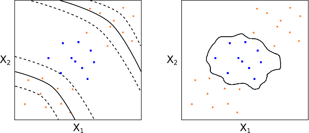
Support Vector Machine decision boundaries for two differing kernels
SVMs are powerful classifiers when used correctly and can provide very promising results. We will now utilise SVMs for the remainder of this article.
Preparing a Dataset for Classification
A famous dataset that is used in machine learning classification design is the Reuters 21578 set. It is one of the most widely used testing datasets for text classification, but it is somewhat out of date these days. However, for the purposes of this article it will more than suffice.
The set consists of a collection of news articles (a "corpus") that are tagged with a selection of topics and geographic locations. Thus it comes "ready made" to be used in classification tests, since it is already pre-labelled.
We will now download, extract and prepare the dataset. I am carrying this tutorial out on a Ubuntu 14.04 machine, so I have access to the command line. If you are on Linux or Mac OSX you will also be able to follow the commands. On Windows, you will need to download a Tar/GZIP extraction tool to get at the data.
The Reuters 21578 dataset can be found from this link as a compressed tar GZIP file. The first task to carry out is to create a new working directory and download the file into it. Please modify the directory name below as you see fit:
cd ~
mkdir -p quantstart/classification/data
cd quantstart/classification/data
wget http://kdd.ics.uci.edu/databases/reuters21578/reuters21578.tar.gz
We can then unzip and untar the file:
tar -zxvf reuters21578.tar.gz
If we list the contents of the directory (ls -l) we can see the following (I have removed the permissions and ownership details for brevity):
...     186 Dec  4  1996 all-exchanges-strings.lc.txt
...     316 Dec  4  1996 all-orgs-strings.lc.txt
...    2474 Dec  4  1996 all-people-strings.lc.txt
...    1721 Dec  4  1996 all-places-strings.lc.txt
...    1005 Dec  4  1996 all-topics-strings.lc.txt
...   28194 Dec  4  1996 cat-descriptions_120396.txt
...  273802 Dec 10  1996 feldman-cia-worldfactbook-data.txt
...    1485 Jan 23  1997 lewis.dtd
...   36388 Sep 26  1997 README.txt
... 1324350 Dec  4  1996 reut2-000.sgm
... 1254440 Dec  4  1996 reut2-001.sgm
... 1217495 Dec  4  1996 reut2-002.sgm
... 1298721 Dec  4  1996 reut2-003.sgm
... 1321623 Dec  4  1996 reut2-004.sgm
... 1388644 Dec  4  1996 reut2-005.sgm
... 1254765 Dec  4  1996 reut2-006.sgm
... 1256772 Dec  4  1996 reut2-007.sgm
... 1410117 Dec  4  1996 reut2-008.sgm
... 1338903 Dec  4  1996 reut2-009.sgm
... 1371071 Dec  4  1996 reut2-010.sgm
... 1304117 Dec  4  1996 reut2-011.sgm
... 1323584 Dec  4  1996 reut2-012.sgm
... 1129687 Dec  4  1996 reut2-013.sgm
... 1128671 Dec  4  1996 reut2-014.sgm
... 1258665 Dec  4  1996 reut2-015.sgm
... 1316417 Dec  4  1996 reut2-016.sgm
... 1546911 Dec  4  1996 reut2-017.sgm
... 1258819 Dec  4  1996 reut2-018.sgm
... 1261780 Dec  4  1996 reut2-019.sgm
... 1049566 Dec  4  1996 reut2-020.sgm
...  621648 Dec  4  1996 reut2-021.sgm
... 8150596 Mar 12  1999 reuters21578.tar.gz
You will see that all the files beginning with reut2- are .sgm, which means that they are SGML files. Unfortunately, Python deprecated sgmllib from Python in 2.6 and fully removed it for Python 3. However, all is not lost because we can create our own SGML Parser class that overrides Python's built in HTMLParser.
Here is a single news item from one of the files:
..
..
<REUTERS TOPICS="YES" LEWISSPLIT="TRAIN" CGISPLIT="TRAINING-SET" OLDID="5544" NEWID="1">
<DATE>26-FEB-1987 15:01:01.79</DATE>
<TOPICS><D>cocoa</D></TOPICS>
<PLACES><D>el-salvador</D><D>usa</D><D>uruguay</D></PLACES>
<PEOPLE></PEOPLE>
<ORGS></ORGS>
<EXCHANGES></EXCHANGES>
<COMPANIES></COMPANIES>
<UNKNOWN>
C T
f0704 reute
u f BC-BAHIA-COCOA-REVIEW 02-26 0105</UNKNOWN>
<TEXT>
<TITLE>BAHIA COCOA REVIEW</TITLE>
<DATELINE> SALVADOR, Feb 26 - </DATELINE><BODY>Showers continued throughout the week in
the Bahia cocoa zone, alleviating the drought since early
January and improving prospects for the coming temporao,
although normal humidity levels have not been restored,
Comissaria Smith said in its weekly review.
The dry period means the temporao will be late this year.
Arrivals for the week ended February 22 were 155,221 bags
of 60 kilos making a cumulative total for the season of 5.93
mln against 5.81 at the same stage last year. Again it seems
that cocoa delivered earlier on consignment was included in the
arrivals figures.
Comissaria Smith said there is still some doubt as to how
much old crop cocoa is still available as harvesting has
practically come to an end. With total Bahia crop estimates
around 6.4 mln bags and sales standing at almost 6.2 mln there
are a few hundred thousand bags still in the hands of farmers,
middlemen, exporters and processors.
There are doubts as to how much of this cocoa would be fit
for export as shippers are now experiencing dificulties in
obtaining +Bahia superior+ certificates.
In view of the lower quality over recent weeks farmers have
sold a good part of their cocoa held on consignment.
Comissaria Smith said spot bean prices rose to 340 to 350
cruzados per arroba of 15 kilos.
Bean shippers were reluctant to offer nearby shipment and
only limited sales were booked for March shipment at 1,750 to
1,780 dlrs per tonne to ports to be named.
New crop sales were also light and all to open ports with
June/July going at 1,850 and 1,880 dlrs and at 35 and 45 dlrs
under New York july, Aug/Sept at 1,870, 1,875 and 1,880 dlrs
per tonne FOB.
Routine sales of butter were made. March/April sold at
4,340, 4,345 and 4,350 dlrs.
April/May butter went at 2.27 times New York May, June/July
at 4,400 and 4,415 dlrs, Aug/Sept at 4,351 to 4,450 dlrs and at
2.27 and 2.28 times New York Sept and Oct/Dec at 4,480 dlrs and
2.27 times New York Dec, Comissaria Smith said.
Destinations were the U.S., Covertible currency areas,
Uruguay and open ports.
Cake sales were registered at 785 to 995 dlrs for
March/April, 785 dlrs for May, 753 dlrs for Aug and 0.39 times
New York Dec for Oct/Dec.
Buyers were the U.S., Argentina, Uruguay and convertible
currency areas.
Liquor sales were limited with March/April selling at 2,325
and 2,380 dlrs, June/July at 2,375 dlrs and at 1.25 times New
York July, Aug/Sept at 2,400 dlrs and at 1.25 times New York
Sept and Oct/Dec at 1.25 times New York Dec, Comissaria Smith
said.
Total Bahia sales are currently estimated at 6.13 mln bags
against the 1986/87 crop and 1.06 mln bags against the 1987/88
crop.
Final figures for the period to February 28 are expected to
be published by the Brazilian Cocoa Trade Commission after
carnival which ends midday on February 27.
Reuter
</BODY></TEXT>
</REUTERS>
..
..
While it may be somewhat laborious to parse data in this manner, especially when compared to the actual machine learning, I can fully reassure you that a large part of a data scientist's or quant researcher's day is in actually getting the data into a format usable by the analysis software! This particular activity is often jokingly referred to as "data wrangling". Hence I feel it is worth it for you to get some practice at it!
If we take a look at the topics file, all-topics-strings.lc.txt, by typing less all-topics-strings.lc.tx we can see the following (I've removed most of it for brevity):
acq
alum
austdlr
austral
barley
bfr
bop
can
carcass
castor-meal
castor-oil
castorseed
citruspulp
cocoa
coconut
coconut-oil
coffee
copper
copra-cake
corn
...
...
silver
singdlr
skr
sorghum
soy-meal
soy-oil
soybean
stg
strategic-metal
sugar
sun-meal
sun-oil
sunseed
tapioca
tea
tin
trade
tung
tung-oil
veg-oil
wheat
wool
wpi
yen
zinc
By calling cat all-topics-strings.lc.txt | wc -l we can see that there are 135 separate topics among the articles. This will make for quite a classification challenge!
At this stage we need to create what is known as a list of predictor-response pairs. This is a list of two-tuples that contain the most appropriate class label and the raw document text, as two separate components. For instance, we wish to end up with a data structure, after parsing, which is similar to the following:
[
    ("cat", "It is best not to give them too much milk"),
    ("dog", "Last night we took him for a walk, but he had to remain on the leash"),
    ..
    ..
    ("hamster", "Today we cleaned out the cage and prepared the sawdust"),
    ("cat", "Kittens require a lot of attention in the first few months")
]
To create this structure we will need to parse all of the Reuters files individually and add them to a grand corpus list. Since the file size of the corpus is rather low, it will easily fit into available RAM on most modern laptops/desktops.
However, in production applications it is usually necessary to stream training data into a machine learning system and carry out "partial fitting" on each batch, in an iterative manner. In later articles we will consider this when we study extremely large data sets (particularly tick data).
As stated above, our first goal is to actually create the SGML Parser that will achieve this. To do this we will subclass Python's HTMLParser class to handle the specific tags in the Reuters dataset.
Upon subclassing HTMLParser we override three methods, handle_starttag, handle_endtag and handle_data, which tell the parser what to do at the beginning of SGML tags, what to do at the closing of SGML tags and how to handle the data in between.
We also create two additional methods, _reset and parse, which are used to take care of internal state of the class and to parse the actual data in a chunked fashion, so as not to use up too much memory.
Finally, I have created a basic __main__ function to test the parser on the first set of data within the Reuters corpus.
As with most, if not all, of the QuantStart code I will comment it verbosely so that you can understand what is going on at every step:
import html
import pprint
import re
from html.parser import HTMLParser


class ReutersParser(HTMLParser):
    """
    ReutersParser subclasses HTMLParser and is used to open the SGML
    files associated with the Reuters-21578 categorised test collection.

    The parser is a generator and will yield a single document at a time.
    Since the data will be chunked on parsing, it is necessary to keep
    some internal state of when tags have been "entered" and "exited".
    Hence the in_body, in_topics and in_topic_d boolean members.
    """
    def __init__(self, encoding='latin-1'):
        """
        Initialise the superclass (HTMLParser) and reset the parser.
        Sets the encoding of the SGML files by default to latin-1.
        """
        html.parser.HTMLParser.__init__(self)
        self._reset()
        self.encoding = encoding

    def _reset(self):
        """
        This is called only on initialisation of the parser class
        and when a new topic-body tuple has been generated. It
        resets all off the state so that a new tuple can be subsequently
        generated.
        """
        self.in_body = False
        self.in_topics = False
        self.in_topic_d = False
        self.body = ""
        self.topics = []
        self.topic_d = ""

    def parse(self, fd):
        """
        parse accepts a file descriptor and loads the data in chunks
        in order to minimise memory usage. It then yields new documents
        as they are parsed.
        """
        self.docs = []
        for chunk in fd:
            self.feed(chunk.decode(self.encoding))
            for doc in self.docs:
                yield doc
            self.docs = []
        self.close()

    def handle_starttag(self, tag, attrs):
        """
        This method is used to determine what to do when the parser
        comes across a particular tag of type "tag". In this instance
        we simply set the internal state booleans to True if that particular
        tag has been found.
        """
        if tag == "reuters":
            pass
        elif tag == "body":
            self.in_body = True
        elif tag == "topics":
            self.in_topics = True
        elif tag == "d":
            self.in_topic_d = True

    def handle_endtag(self, tag):
        """
        This method is used to determine what to do when the parser
        finishes with a particular tag of type "tag".

        If the tag is a <REUTERS> tag, then we remove all
        white-space with a regular expression and then append the
        topic-body tuple.

        If the tag is a <BODY> or <TOPICS> tag then we simply set
        the internal state to False for these booleans, respectively.

        If the tag is a <D> tag (found within a <TOPICS> tag), then we
        append the particular topic to the "topics" list and
        finally reset it.
        """
        if tag == "reuters":
            self.body = re.sub(r'\s+', r' ', self.body)
            self.docs.append( (self.topics, self.body) )
            self._reset()
        elif tag == "body":
            self.in_body = False
        elif tag == "topics":
            self.in_topics = False
        elif tag == "d":
            self.in_topic_d = False
            self.topics.append(self.topic_d)
            self.topic_d = ""

    def handle_data(self, data):
        """
        The data is simply appended to the appropriate member state
        for that particular tag, up until the end closing tag appears.
        """
        if self.in_body:
            self.body += data
        elif self.in_topic_d:
            self.topic_d += data


if __name__ == "__main__":
    # Open the first Reuters data set and create the parser
    filename = "data/reut2-000.sgm"
    parser = ReutersParser()

    # Parse the document and force all generated docs into
    # a list so that it can be printed out to the console
    doc = parser.parse(open(filename, 'rb'))
    pprint.pprint(list(doc))
At this stage we will see a significant amount of output that looks like this:
..
..
(['grain', 'rice', 'thailand'],
  'Thailand exported 84,960 tonnes of rice in the week ended February 24, '
  'up from 80,498 the previous week, the Commerce Ministry said. It said '
  'government and private exporters shipped 27,510 and 57,450 tonnes '
  'respectively. Private exporters concluded advance weekly sales for '
  '79,448 tonnes against 79,014 the previous week. Thailand exported '
  '689,038 tonnes of rice between the beginning of January and February 24, '
  'up from 556,874 tonnes during the same period last year. It has '
  'commitments to export another 658,999 tonnes this year. REUTER '),
 (['soybean', 'red-bean', 'oilseed', 'japan'],
  'The Tokyo Grain Exchange said it will raise the margin requirement on '
  'the spot and nearby month for U.S. And Chinese soybeans and red beans, '
  'effective March 2. Spot April U.S. Soybean contracts will increase to '
  '90,000 yen per 15 tonne lot from 70,000 now. Other months will stay '
  'unchanged at 70,000, except the new distant February requirement, which '
  'will be set at 70,000 from March 2. Chinese spot March will be set at '
  '110,000 yen per 15 tonne lot from 90,000. The exchange said it raised '
  'spot March requirement to 130,000 yen on contracts outstanding at March '
  '13. Chinese nearby April rises to 90,000 yen from 70,000. Other months '
  'will remain unchanged at 70,000 yen except new distant August, which '
  'will be set at 70,000 from March 2. The new margin for red bean spot '
  'March rises to 150,000 yen per 2.4 tonne lot from 120,000 and to 190,000 '
  'for outstanding contracts as of March 13. The nearby April requirement '
  'for red beans will rise to 100,000 yen from 60,000, effective March 2. '
  'The margin money for other red bean months will remain unchanged at '
  '60,000 yen, except new distant August, for which the requirement will '
  'also be set at 60,000 from March 2. REUTER '),
..
..
In particular, note that instead of having a single topic label associated with a document, we have multiple topics. In order to increase the effectiveness of the classifier, it is necessary to assign only a single class label to each document. However, you'll also note that some of the labels are actually geographic location tags, such as "japan" or "thailand". Since we are concerned solely with topics and not countries we want to remove these before we select our topic.
The particular method that we will use to carry this out is rather simple. We will strip out the country names and then select the first remaining topic on the list. If there are no associated topics we will eliminate the article from our corpus. In the above output, this will reduce to a data structure that looks like:
..
..
 ('grain',
  'Thailand exported 84,960 tonnes of rice in the week ended February 24, '
  'up from 80,498 the previous week, the Commerce Ministry said. It said '
  'government and private exporters shipped 27,510 and 57,450 tonnes '
  'respectively. Private exporters concluded advance weekly sales for '
  '79,448 tonnes against 79,014 the previous week. Thailand exported '
  '689,038 tonnes of rice between the beginning of January and February 24, '
  'up from 556,874 tonnes during the same period last year. It has '
  'commitments to export another 658,999 tonnes this year. REUTER '),
 ('soybean',
  'The Tokyo Grain Exchange said it will raise the margin requirement on '
  'the spot and nearby month for U.S. And Chinese soybeans and red beans, '
  'effective March 2. Spot April U.S. Soybean contracts will increase to '
  '90,000 yen per 15 tonne lot from 70,000 now. Other months will stay '
  'unchanged at 70,000, except the new distant February requirement, which '
  'will be set at 70,000 from March 2. Chinese spot March will be set at '
  '110,000 yen per 15 tonne lot from 90,000. The exchange said it raised '
  'spot March requirement to 130,000 yen on contracts outstanding at March '
  '13. Chinese nearby April rises to 90,000 yen from 70,000. Other months '
  'will remain unchanged at 70,000 yen except new distant August, which '
  'will be set at 70,000 from March 2. The new margin for red bean spot '
  'March rises to 150,000 yen per 2.4 tonne lot from 120,000 and to 190,000 '
  'for outstanding contracts as of March 13. The nearby April requirement '
  'for red beans will rise to 100,000 yen from 60,000, effective March 2. '
  'The margin money for other red bean months will remain unchanged at '
  '60,000 yen, except new distant August, for which the requirement will '
  'also be set at 60,000 from March 2. REUTER '),
..
..
To remove the geographic tags and select the primary topic tag we can add the following code:
..
..

def obtain_topic_tags():
    """
    Open the topic list file and import all of the topic names
    taking care to strip the trailing "\n" from each word.
    """
    topics = open(
        "data/all-topics-strings.lc.txt", "r"
    ).readlines()
    topics = [t.strip() for t in topics]
    return topics

def filter_doc_list_through_topics(topics, docs):
    """
    Reads all of the documents and creates a new list of two-tuples
    that contain a single feature entry and the body text, instead of
    a list of topics. It removes all geographic features and only
    retains those documents which have at least one non-geographic
    topic.
    """
    ref_docs = []
    for d in docs:
        if d[0] == [] or d[0] == "":
            continue
        for t in d[0]:
            if t in topics:
                d_tup = (t, d[1])
                ref_docs.append(d_tup)
                break
    return ref_docs


if __name__ == "__main__":
    # Open the first Reuters data set and create the parser
    filename = "data/reut2-000.sgm"
    parser = ReutersParser()

    # Parse the document and force all generated docs into
    # a list so that it can be printed out to the console
    docs = list(parser.parse(open(filename, 'rb')))

    # Obtain the topic tags and filter docs through it
    topics = obtain_topic_tags()
    ref_docs = filter_doc_list_through_topics(topics, docs)
    pprint.pprint(ref_docs)
The output from this is as follows:
..
..
('acq',
  'Security Pacific Corp said it completed its planned merger with Diablo '
  'Bank following the approval of the comptroller of the currency. Security '
  'Pacific announced its intention to merge with Diablo Bank, headquartered '
  'in Danville, Calif., in September 1986 as part of its plan to expand its '
  'retail network in Northern California. Diablo has a bank offices in '
  'Danville, San Ramon and Alamo, Calif., Security Pacific also said. '
  'Reuter '),
 ('earn',
  'Shr six cts vs five cts Net 188,000 vs 130,000 Revs 12.2 mln vs 10.1 mln '
  'Avg shrs 3,029,930 vs 2,764,544 12 mths Shr 81 cts vs 1.45 dlrs Net '
  '2,463,000 vs 3,718,000 Revs 52.4 mln vs 47.5 mln Avg shrs 3,029,930 vs '
  '2,566,680 NOTE: net for 1985 includes 500,000, or 20 cts per share, for '
  'proceeds of a life insurance policy. includes tax benefit for prior qtr '
  'of approximately 150,000 of which 140,000 relates to a lower effective '
  'tax rate based on operating results for the year as a whole. Reuter '),
..
..
We are now in a position to pre-process the data for input into the classifier.
Vectorisation
At this stage we have a large collection of two-tuples, each containing a class label and raw body text from the articles. The obvious question to ask now is how do we convert the raw body text into a data representation that can be used by a (numerical) classifier?
The answer lies in a process known as vectorisation. Vectorisation allows widely-varying lengths of raw text to be converted into a numerical format that can be processed by the classifier.
It achieves this by creating tokens from a string. A token is an individual word (or group of words) extracted from a document, using whitespace or punctuation as separators. This can, of course, include numbers from within the string as additional "words". Once this list of tokens has been created they can be assigned an integer identifier, which allows them to be listed.
Once the list of tokens have been generated, the number of tokens within a document are counted. Finally, these tokens are normalised to de-emphasise tokens that appear frequently within a document (such as "a", "the"). This process is known as the Bag Of Words.
The Bag Of Words representation allows a vector to be associated with each document, each component of which is real-valued and represents the importance of tokens (i.e. "words") appearing within that document.
Further, it means that once an entire corpus of documents has been iterated over (and thus all possible tokens have been assessed), the total number of separate tokens is known and hence the length of the token vector, for any document of any length is also fixed and identical.
This means that the classifier now has a set of features via the frequency of token occurance. In addition the document token-vector represents a sample for the classifier.
In essence, the entire corpus can be represented as a large matrix, each row of which represents one of the documents and each column represents token occurance within that document. This is the process of vectorisation.
Note that vectorisation does not take into account the relative positioning of the words within the document, just the frequency of occurance. More sophisticated machine learning techniques will, however, use this information to enhance classification.
Term-Frequency Inverse Document-Frequency
One of the major issues with vectorisation, via the Bag Of Words representation, is that there is a lot of "noise" in the form of stop words, such as "a", "the", "he", "she" etc. These words provide little context to the document but their high frequency will mean that they can mask words that do provide document context.
This motivates a transformation process, known as Term-Frequency Inverse Document-Frequency (TF-IDF). The TF-IDF value for a token increases proportionally to the frequency of the word in the document but is normalised by the frequency of the word in the corpus. This essentially reduces importance for words that appear a lot generally, as opposed to appearing a lot within a particular document.
This is precisely what we need as words such as "a", "the" will have extremely high occurances within the entire corpus, but the word "cat" may only appear often in a particular document. This would mean that we are giving "cat" a relatively higher strength than "a" or "the", for that document.
I won't dwell on the calculation of TF-IDF, but if you are interested then read the Wikipedia article on the subject, which goes into more detail.
Hence we wish to combine the process of vectorisation with that of TF-IDF to produce a normalised matrix of document-token occurances. This will then be used to provide a list of features to the classifier upon which to train.
Thankfully, the developers at scikit-learn realised that it would be an extremely common operation to vectorise and transform text files in this manner and so included the TfidfVectorizer class.
We can use this class to take our list of two-tuples representing class labels and raw document text, to produce both a vector of class labels and a sparse matrix, which represents the TF-IDF and Vectorisation procedure applied to the raw text data.
Since scikit-learn classifiers take two separate data structures for training, namely, $y$, the vector of class labels or "responses" associated with an ordered set of documents, and, $X$, the sparse TF-IDF matrix of raw document text, we modify our two-tuple list to create $y$ and $X$. The code to create these objects is given below:
..
from sklearn.feature_extraction.text import TfidfVectorizer
..
..

def create_tfidf_training_data(docs):
    """
    Creates a document corpus list (by stripping out the
    class labels), then applies the TF-IDF transform to this
    list.

    The function returns both the class label vector (y) and
    the corpus token/feature matrix (X).
    """
    # Create the training data class labels
    y = [d[0] for d in docs]

    # Create the document corpus list
    corpus = [d[1] for d in docs]

    # Create the TF-IDF vectoriser and transform the corpus
    vectorizer = TfidfVectorizer(min_df=1)
    X = vectorizer.fit_transform(corpus)
    return X, y


if __name__ == "__main__":
    # Open the first Reuters data set and create the parser
    filename = "data/reut2-000.sgm"
    parser = ReutersParser()

    # Parse the document and force all generated docs into
    # a list so that it can be printed out to the console
    docs = list(parser.parse(open(filename, 'rb')))

    # Obtain the topic tags and filter docs through it
    topics = obtain_topic_tags()
    ref_docs = filter_doc_list_through_topics(topics, docs)

    # Vectorise and TF-IDF transform the corpus
    X, y = create_tfidf_training_data(ref_docs)
At this stage we now have two components to our training data. The first, $X$, is a matrix of document-token occurances. The second, $y$, is a vector (which matches the ordering of the matrix) that contains the correct class labels for each of the documents. This is all we need to begin training and testing the Support Vector Machine.
Training the Support Vector Machine
In order to train the Support Vector Machine it is necessary to provide it with both a set of features (the $X$ matrix) and a set of "supervised" training labels, in this case the $y$ classes. However, we also need a means of evaluating the trained performance of the classifier subsequent to its training phase.
One approach is to simply try classifying some of the documents from the corpus used to train it on. Such an evaluation procedure is known as in-sample testing. However, this is not a particularly effective mechanism for assessing the performance of the system.
Simply put, the classifier has already "seen" this data and has been told how to act upon it and so it is very likely to correctly classify the document. This will almost certainly overstate the classifier's true out-of-sample testing performance. Hence we need to provide the classifier with data that it has not used for training, as a more realistic means of testing.
However, it is not obvious where to obtain this new data from. One approach might be to create a separate corpus from some new data. However, in reality this is likely to be expensive in terms of time and/or business processes. An alternative approach is to partition the training set into two distinct subsets, one of which is used for training and the other for testing. This is known as the training-test split.
Such a partition allows us to train the classifier solely on the first partition and then classify its performance on the second partition. This gives us a much better insight into how it will perform in true "out-of-sample" data going forward.
One question that arises here is what percentage to retain for training and what to use for testing. Clearly the more that is retained for training, the "better" the classifier will be because it will have seen more data. However, more training data means less testing data and as such a poorer estimate of its true classification capability. In practice, it is common to retain about 70-80% of the data for training and use the remainder for testing.
Since the training-test split is such a common operation in machine learning, the developers of scikit-learn provided the train_test_split method to automatically create the split from a dataset provided. Here is the code that provides the split:
from sklearn.cross_validation import train_test_split
..
..
X_train, X_test, y_train, y_test = train_test_split(
  X, y, test_size=0.2, random_state=42
)
The test_size keyword argument controls the size of the testing set, in this case 20%. The random_state keyword argument controls the random seed for selecting the partition randomly.
The next step is to actually create the Support Vector Machine and train it. In this instance we are going to use the SVC (Support Vector Classifier) class from scikit-learn. We give it the parameters $C=1000000.0$, $\gamma=0.0$ and choose a radial kernel. To understand where these parameters come from, please take a look at the article on Support Vector Machines.
The following code imports the SVC class and then fits it on the training data:
from sklearn.svm import SVC
..
..
def train_svm(X, y):
    """
    Create and train the Support Vector Machine.
    """
    svm = SVC(C=1000000.0, gamma=0.0, kernel='rbf')
    svm.fit(X, y)
    return svm


if __name__ == "__main__":
    # Open the first Reuters data set and create the parser
    filename = "data/reut2-000.sgm"
    parser = ReutersParser()

    # Parse the document and force all generated docs into
    # a list so that it can be printed out to the console
    docs = list(parser.parse(open(filename, 'rb')))

    # Obtain the topic tags and filter docs through it
    topics = obtain_topic_tags()
    ref_docs = filter_doc_list_through_topics(topics, docs)

    # Vectorise and TF-IDF transform the corpus
    X, y = create_tfidf_training_data(ref_docs)

    # Create the training-test split of the data
    X_train, X_test, y_train, y_test = train_test_split(
        X, y, test_size=0.2, random_state=42
    )

    # Create and train the Support Vector Machine
    svm = train_svm(X_train, y_train)
Now that the SVM has been trained we need to assess its performance on the testing data.
Performance Metrics
The two main performance metrics that we will consider for this supervised classifer are the hit-rate and the confusion matrix. The former is simply the ratio of correct assignments to total assignments and is usually quoted as a percentage.
The confusion matrix goes into more detail and provides output on true-positives, true-negatives, false-positives and false-negatives. In a binary classification system, with a "true" or "false" class labelling, these characterise the rate at which the classifier correctly classifies something as true or false when it is, respectively, true or false, and also incorrectly classifies something as true or false when it is, respectively, false or true.
A confusion matrix need not be restricted to a binary classifier situation. For multiple class groups (as in our situation with the Reuters dataset) we will have an $N \times N$ matrix, where $N$ is the number of class labels (or document topics).
Scikit-learn has functions for calculating both the hit-rate and the confusion matrix of a supervised classifier. The former is a method on the classifier itself called score. The latter must be imported from the metrics library.
The first task is to create a predictions array from the X_test test-set. This will simply contain the predicted class labels from the SVM via the retained 20% test set. This prediction array is used to create the confusion matrix. Notice that the confusion_matrix function takes both the pred predictions array and the y_test correct class labels to produce the matrix. In addition we create the hit-rate by providing score with both the X_test and y_test subsets of the dataset:
..
..
from sklearn.metrics import confusion_matrix
..
..


if __name__ == "__main__":

    ..
    ..

    # Create and train the Support Vector Machine
    svm = train_svm(X_train, y_train)

    # Make an array of predictions on the test set
    pred = svm.predict(X_test)

    # Output the hit-rate and the confusion matrix for each model
    print(svm.score(X_test, y_test))
    print(confusion_matrix(pred, y_test))
The output of the code is as follows:
0.660194174757
[[21  0  0  0  2  3  0  0  0  1  0  0  0  0  1  1  1  0  0]
 [ 0  0  0  0  0  0  0  0  0  0  0  0  0  0  0  0  0  0  0]
 [ 0  0  1  0  0  0  0  0  0  0  0  0  0  0  0  0  0  0  0]
 [ 0  0  0  1  0  0  0  0  0  0  0  0  0  0  0  0  0  0  0]
 [ 0  0  0  0  4  0  0  0  0  0  0  0  0  0  0  0  0  0  0]
 [ 0  1  0  0  1 26  0  0  0  1  0  1  0  1  0  0  0  0  0]
 [ 0  0  0  0  0  0  2  0  0  0  0  0  0  0  0  0  0  0  1]
 [ 0  0  0  0  0  0  0  1  0  0  0  0  0  0  0  0  0  0  0]
 [ 0  0  0  0  0  0  0  0  0  0  0  0  0  0  0  0  0  0  0]
 [ 0  0  0  0  1  0  0  0  0  3  0  0  0  0  0  0  0  0  0]
 [ 3  0  0  1  2  2  3  0  1  1  6  0  1  0  0  0  2  3  0]
 [ 0  0  0  0  0  0  0  0  0  0  0  0  0  0  0  0  0  0  0]
 [ 0  0  0  0  0  0  0  0  0  0  0  0  0  0  0  0  0  0  0]
 [ 0  0  0  0  0  0  0  0  0  0  0  0  0  1  0  0  0  0  0]
 [ 0  0  0  0  0  0  0  0  0  0  0  0  0  0  1  0  0  0  0]
 [ 0  0  0  0  0  0  0  0  0  0  0  0  0  0  0  1  0  0  0]
 [ 0  0  0  0  0  0  0  0  0  0  0  0  0  0  0  0  0  0  0]
 [ 0  0  0  0  0  0  0  0  0  0  0  0  0  0  0  0  0  0  0]
 [ 0  0  0  0  0  0  0  0  0  0  0  0  0  0  0  0  0  0  0]]
Thus we have a 66% classification hit rate, with a confusion matrix that has entries mainly on the diagonal (i.e. the correct assignment of class label). Notice that since we are only using a single file from the Reuters set (number 000), we aren't going to see the entire set of class labels and hence our confusion matrix is smaller in dimension than if we had used the full dataset.
In order to make use of the full dataset we can modify the __main__ function to load all 21 Reuters files and train the SVM on the full dataset. We can output the full hit-rate performance. I've neglected to include the confusion matrix output as it becomes large for the total number of class labels within all documents. Note that this will take some time! On my system it takes about 30-45 seconds to run.
if __name__ == "__main__":
    # Create the list of Reuters data and create the parser
    files = ["data/reut2-%03d.sgm" % r for r in range(0, 22)]
    parser = ReutersParser()

    # Parse the document and force all generated docs into
    # a list so that it can be printed out to the console
    docs = []
    for fn in files:
        for d in parser.parse(open(fn, 'rb')):
            docs.append(d)

    ..
    ..

    print(svm.score(X_test, y_test))
For the full corpus, the hit rate provided is 83.6%:
0.835971855761
There are plenty of ways to improve on this figure. In particular we can perform a Grid Search Cross-Validation, which is a means of determining the optimal parameters for the classifier that will achieve the best hit-rate (or other metric of choice).
In later articles we will discuss such optimisation procedures and explain how a classifier such as this can be added to a production system in a data science or quantitative finance context.
Full Code Implementation in Python 3.4.x
Here is the full code for reuters_svm.py written in Python 3.4.x:
import html
import pprint
import re
from html.parser import HTMLParser

from sklearn.cross_validation import train_test_split
from sklearn.feature_extraction.text import TfidfVectorizer
from sklearn.metrics import confusion_matrix
from sklearn.svm import SVC


class ReutersParser(HTMLParser):
    """
    ReutersParser subclasses HTMLParser and is used to open the SGML
    files associated with the Reuters-21578 categorised test collection.

    The parser is a generator and will yield a single document at a time.
    Since the data will be chunked on parsing, it is necessary to keep
    some internal state of when tags have been "entered" and "exited".
    Hence the in_body, in_topics and in_topic_d boolean members.
    """
    def __init__(self, encoding='latin-1'):
        """
        Initialise the superclass (HTMLParser) and reset the parser.
        Sets the encoding of the SGML files by default to latin-1.
        """
        html.parser.HTMLParser.__init__(self)
        self._reset()
        self.encoding = encoding

    def _reset(self):
        """
        This is called only on initialisation of the parser class
        and when a new topic-body tuple has been generated. It
        resets all off the state so that a new tuple can be subsequently
        generated.
        """
        self.in_body = False
        self.in_topics = False
        self.in_topic_d = False
        self.body = ""
        self.topics = []
        self.topic_d = ""

    def parse(self, fd):
        """
        parse accepts a file descriptor and loads the data in chunks
        in order to minimise memory usage. It then yields new documents
        as they are parsed.
        """
        self.docs = []
        for chunk in fd:
            self.feed(chunk.decode(self.encoding))
            for doc in self.docs:
                yield doc
            self.docs = []
        self.close()

    def handle_starttag(self, tag, attrs):
        """
        This method is used to determine what to do when the parser
        comes across a particular tag of type "tag". In this instance
        we simply set the internal state booleans to True if that particular
        tag has been found.
        """
        if tag == "reuters":
            pass
        elif tag == "body":
            self.in_body = True
        elif tag == "topics":
            self.in_topics = True
        elif tag == "d":
            self.in_topic_d = True

    def handle_endtag(self, tag):
        """
        This method is used to determine what to do when the parser
        finishes with a particular tag of type "tag".

        If the tag is a  tag, then we remove all
        white-space with a regular expression and then append the
        topic-body tuple.

        If the tag is a  or  tag then we simply set
        the internal state to False for these booleans, respectively.

        If the tag is a  tag (found within a  tag), then we
        append the particular topic to the "topics" list and
        finally reset it.
        """
        if tag == "reuters":
            self.body = re.sub(r'\s+', r' ', self.body)
            self.docs.append( (self.topics, self.body) )
            self._reset()
        elif tag == "body":
            self.in_body = False
        elif tag == "topics":
            self.in_topics = False
        elif tag == "d":
            self.in_topic_d = False
            self.topics.append(self.topic_d)
            self.topic_d = ""

    def handle_data(self, data):
        """
        The data is simply appended to the appropriate member state
        for that particular tag, up until the end closing tag appears.
        """
        if self.in_body:
            self.body += data
        elif self.in_topic_d:
            self.topic_d += data


def obtain_topic_tags():
    """
    Open the topic list file and import all of the topic names
    taking care to strip the trailing "\n" from each word.
    """
    topics = open(
        "data/all-topics-strings.lc.txt", "r"
    ).readlines()
    topics = [t.strip() for t in topics]
    return topics

def filter_doc_list_through_topics(topics, docs):
    """
    Reads all of the documents and creates a new list of two-tuples
    that contain a single feature entry and the body text, instead of
    a list of topics. It removes all geographic features and only
    retains those documents which have at least one non-geographic
    topic.
    """
    ref_docs = []
    for d in docs:
        if d[0] == [] or d[0] == "":
            continue
        for t in d[0]:
            if t in topics:
                d_tup = (t, d[1])
                ref_docs.append(d_tup)
                break
    return ref_docs

def create_tfidf_training_data(docs):
    """
    Creates a document corpus list (by stripping out the
    class labels), then applies the TF-IDF transform to this
    list.

    The function returns both the class label vector (y) and
    the corpus token/feature matrix (X).
    """
    # Create the training data class labels
    y = [d[0] for d in docs]

    # Create the document corpus list
    corpus = [d[1] for d in docs]

    # Create the TF-IDF vectoriser and transform the corpus
    vectorizer = TfidfVectorizer(min_df=1)
    X = vectorizer.fit_transform(corpus)
    return X, y

def train_svm(X, y):
    """
    Create and train the Support Vector Machine.
    """
    svm = SVC(C=1000000.0, gamma=0.0, kernel='rbf')
    svm.fit(X, y)
    return svm


if __name__ == "__main__":
    # Create the list of Reuters data and create the parser
    files = ["data/reut2-%03d.sgm" % r for r in range(0, 22)]
    parser = ReutersParser()

    # Parse the document and force all generated docs into
    # a list so that it can be printed out to the console
    docs = []
    for fn in files:
        for d in parser.parse(open(fn, 'rb')):
            docs.append(d)

    # Obtain the topic tags and filter docs through it
    topics = obtain_topic_tags()
    ref_docs = filter_doc_list_through_topics(topics, docs)

    # Vectorise and TF-IDF transform the corpus
    X, y = create_tfidf_training_data(ref_docs)

    # Create the training-test split of the data
    X_train, X_test, y_train, y_test = train_test_split(
        X, y, test_size=0.2, random_state=42
    )

    # Create and train the Support Vector Machine
    svm = train_svm(X_train, y_train)

    # Make an array of predictions on the test set
    pred = svm.predict(X_test)

    # Output the hit-rate and the confusion matrix for each model
    print(svm.score(X_test, y_test))
    print(confusion_matrix(pred, y_test))


