To date QuantStart has generally written on topics that are applicable to the beginner or intermediate quant practitioner. However we have recently begun to receive requests from academics and advanced practitioners asking for more content on research-level topics.
This is the first in a new series of posts written by Imanol Pérez, a PhD researcher in Mathematics at Oxford University, UK, and a new expert guest contributor to QuantStart. In this introductory post Imanol describes the Theory of Rough Paths, applying Python to compute the Lead-Lag and Time-Joined transformations to a stream of IBM pricing data.
- Mike.
Since the theory of rough paths was introduced in the late 90s[5], the field has evolved considerably and at a very fast pace. Moreover, in the last few years there have been many papers[3], [2], [1] showing how to apply rough path theory to machine learning and time series analysis.
Rough path theory, as the name suggests, deals with paths (that is, continuous functions $X:[0,T]\rightarrow \mathbb{R}^d$) that are rough, in the sense of being highly oscillatory. In this article, we will introduce the theory of rough paths from a theoretical point of view. This introduction will be followed by several articles that will show, with concrete examples, how some of the results that are stated here can be used in quantitative finance.
Tensor algebra
Before defining the signature of a continuous path and introducing its properties, we shall define the tensor algebra space we will be dealing with. The $n$-th tensor power of $\mathbb{R}^d$ is defined as
\begin{equation*} (\mathbb{R}^d)^{\otimes n} := \underbrace{\mathbb{R}^d\otimes \mathbb{R}^d\otimes \ldots \otimes \mathbb{R}^d}_n, \end{equation*} where $\otimes$ is the tensor product. We define the tensor algebra space as
\begin{equation} T((\mathbb{R}^d)):=\{(a_0, a_1, a_2, \ldots) : a_n \in (\mathbb{R}^d)^{\otimes n} \mbox{ }\forall n\geq 0\}, \end{equation} were we take $(\mathbb{R}^d)^{\otimes 0}=\mathbb{R}$ by convention. Moreover, we shall also introduce the truncated tensor algebra space $T^n(E)$, which is defined as
\begin{equation}\label{eq:truncated tensor algebra 1} T^n(\mathbb{R}^d):=\bigoplus_{i=0}^n (\mathbb{R}^d)^{\otimes i}. \end{equation}
Given two elements $a=(a_0,a_1,\ldots),b=(b_0,b_1,\ldots)\in T((\mathbb{R}^d))$, we may introduce the sum and product of $a$ and $b$ as
\begin{equation*} a+b:=(a_0+b_0, a_1+b_1, a_2+b_2,\ldots), \end{equation*}\begin{equation*} a\otimes b=ab:=\left (\sum_{i=0}^n a_i \otimes b_{n-i} \right )_{n\geq 0}. \end{equation*}
Summation and multiplication in the truncated tensor algebra can be defined analogously.
Signature of a path
The signature of a path is a key object in the theory of rough paths. For a continuous path $X:[0,T]\rightarrow \mathbb{R}^d$ such that the integrals below make sense, the signature of $X$ is defined as the sequence
$$S(X):=(1,X^1,X^2,\ldots)\in T((\mathbb{R}^d))$$
where
$$X^n := \underset{\substack{0 < u_1 < u_2 < \ldots < u_n < T}}{\int\ldots\int} dX_{u_1} \otimes \ldots \otimes dX_{u_n} \in (\mathbb{R}^d)^{\otimes n}\quad \forall n \geq 1.$$
Sometimes we are only interested in the truncated signature, which is defined as
$$S^n(X):=(1,X^1,X^2,\ldots,X^n).$$
The signature of a path can also be defined as the sequence $(X^I)_{I\in \mathcal{I}}$, where $\mathcal{I}$ is the set of all multi-indices with entries in $\{1,\ldots,d\}$, and $X^I$ is defined, for $I=(i_1,\ldots,i_n)$, as the iterated integral
\begin{equation}\label{eq:alternative signature} X^I = \underset{\substack{0 < u_1 < u_2 < \ldots < u_n < T}}{\int\ldots\int} dX_{u_1}^{i_1} \ldots dX_{u_n}^{i_n}. \end{equation}
This way of expressing the signature allows to have a better intuition of it, and how it may be calculated in practice. Let us take a closer look to what the iterated integrals look like for the low order terms, for instance. Take the above equation with $I=(i)$, for $i=1,\ldots,d$. Then, $X^{(i)}=X_T^i-X_0^i$, that is, the first order terms of the signature are nothing else than the increments of the path.
For the second order iterated integral, let us consider $I=(i,j)$, with $i,j\in \{1,\ldots,d\}$ not necessarily distinct. Then, we have
\begin{equation*} \begin{split} \left ( \int_{0}^T dX_{u_1}^{i}\right ) \left ( \int_{0}^T dX_{u_2}^{j} \right )=\underset{\substack{u_1, u_2 \in [0,T]}}{\int} dX_{u_1}^{i}dX_{u_2}^{j} = \\ =\underset{\substack{0 < u_1 < u_2 < T}}{\int} dX_{u_1}^{i}dX_{u_2}^{j}+\underset{\substack{0 < u_2 < u_1 < T}}{\int} dX_{u_1}^{i}dX_{u_2}^{j}. \end{split} \end{equation*}
That is, we have the following identity:
\begin{equation}\label{eq:identity second order signature} X^{(i,j)}+X^{(j,i)}=X^{(i)}X^{(j)}\quad \forall i,j\in \{1,\ldots,d\}, \end{equation} and in particular, letting $i=j$,
\begin{equation} X^{(i,i)}=\dfrac{\left (X^{(i)}\right )^2}{2} \quad \forall i=1,\ldots,d. \end{equation}
The equation shows how the first and second order terms are related in the signature.
Signature of a stream of data
In the previous section we defined the signature of a continuous path. However, in real life we cannot observe a full continuous path, we can only expect to observe a stream of data that consists of a sampling of the path we are interested in. In financial securities, for instance, the market only shows the prices of the securities at specific times. Therefore, in order to apply techniques from rough path theory to financial securities, we need to define what we mean by the signature of a stream of data.
Mathematically, a stream of data (which for now will be assumed to be one dimensional) is denoted by $\{(t, S_t)\}_{t\in \mathcal{D}}$, where $\mathcal{D}\subset [0,T]$ is the times at which information about the path is available, and $S_t$ denotes the value of the path at time $t$. In financial terms, $\mathcal{D}$ denotes the times at which we have information about the price of a security, and $S_t$ denotes the price of the security at time $t$.
The way to proceed in this case is quite simple: we first transform the stream of data into a continuous path, and then calculate the signature of this new path. We will show two approaches for this task: the lead-lag transformation, and the time-joined transformation. In both cases the resulting continuous path is piecewise linear, which makes the calculation of the signature easier and computationally fast[3].
Lead-lag transformation
As mentioned, we want to transform the stream of data $\{(t, S_t)\}_{t\in \mathcal{D}}$ into a continuous path. If $\mathcal{D}$ is given by the times $0\leq t_0 < t_1 < \ldots < t_N \leq T$, we may then write the stream of data as
$$\{(t_i, S_{t_i})\}_{i=0}^N.$$
Then, the lead-lag transformation of the stream of data is defined as
\begin{align*} \widehat{S}_t^\mathcal{D}:= \begin{cases} (S_{t_i}, S_{t_{i+1}})&\mbox{for }t\in [2i, 2i+1)\\ (S_{t_i}, S_{t_{i+1}}+2(t-(2i+1))(S_{t_{i+2}}-S_{t_{i+1}})&\mbox{for }t\in \left [2i+1, 2i+\frac{3}{2}\right )\\ (S_{t_i}+2\left (t-\left (2i+\frac{3}{2}\right )\right )(S_{t_{i+1}}-S_{t_i}), S_{t_{i+2}})&\mbox{for }t\in \left [2i+\frac{3}{2}, 2i+2\right ). \end{cases}, \end{align*} for $t\in [0, 2N]$. As we see, this path is $2$-dimensional, and we often write it as $\widehat{S}^\mathcal{D}=(\widehat{S}^{\mathcal{D},b}, \widehat{S}^{\mathcal{D},f})$. The first term, $\widehat{X}^{\mathcal{D}, b}$, corresponds to the lead component and the second term, $\widehat{X}^{\mathcal{D}, f}$, corresponds to the lag component.
The following code, implemented in Python, computes and plots the lead-lag transformation of a stream of data:
import matplotlib.pyplot as plt
import matplotlib.dates as mdates
import matplotlib.patches as patches

def leadlag(X):
    '''
    Returns lead-lag-transformed stream of X

    Arguments:
        X: list, whose elements are tuples of the form
        (time, value).

    Returns:
        list of points on the plane, the lead-lag
        transformed stream of X
    '''

    l=[]

    for j in range(2*(len(X))-1):
        i1=j//2
        i2=j//2
        if j%2!=0:
            i1+=1
        l.append((X[i1][1], X[i2][1]))

    return l

def plotLeadLag(X, diagonal=True):
    '''
    Plots the lead-laged transformed path X. If diagonal
    is True, a line joining the start and ending points
    is displayed.

    Arguments:
        X: list, whose elements are tuples of the form
        (X^lead, X^lag) diagonal: boolean, default is
        True. If True, a line joining the start and
        ending points is displayed.
    '''
    for i in range(len(X)-1):
        plt.plot([X[i][1], X[i+1][1]], [X[i][0], X[i+1][0]],
                    color='k', linestyle='-', linewidth=2)


    # Show the diagonal, if diagonal is true
    if diagonal:
        plt.plot([min(min([p[0] for p in X]), min([p[1]
                for p in X])), max(max([p[0] for p in X]),
                max([p[1] for p in X]))], [min(min([p[0]
                for p in X]), min([p[1] for p in X])),
                max(max([p[0] for p in X]), max([p[1] for
                p in X]))], color='#BDBDBD', linestyle='-',
                linewidth=1)

    axes=plt.gca()
    axes.set_xlim([min([p[1] for p in X])-1, max([p[1] for
                  p in X])+1])
    axes.set_ylim([min([p[0] for p in X])-1, max([p[0] for
                  p in X])+1])
    axes.get_yaxis().get_major_formatter().set_useOffset(False)
    axes.get_xaxis().get_major_formatter().set_useOffset(False)
    axes.set_aspect('equal', 'datalim')
    plt.show()
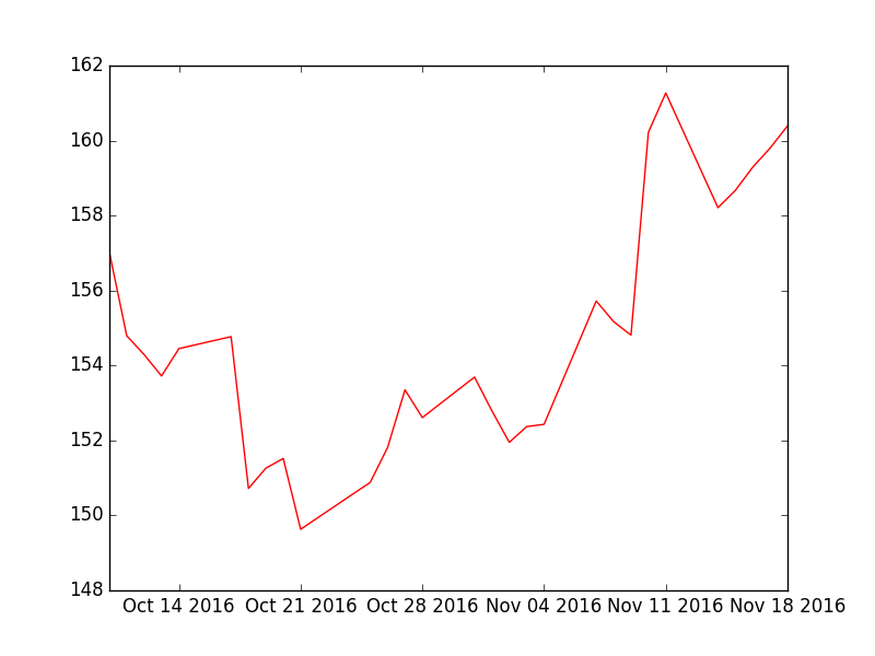
Fig 1 - Path of IBM stock
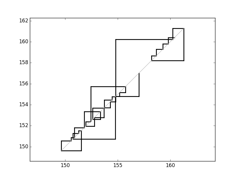
Fig 2 - Lead-lag transformation of IBM stock
Figures 1 and 2 show the price of IBM's stock from October 2016 to November 2016, and its lead-lag transformation, which was computed using the code above.
Time-joined transformation
An alternative way of transforming the stream of data $\{(t_i, S_{t_i}\}_{i=0}^N$ into a continuous path is using the time-joined transformation, which is defined as
\begin{align*} Y_t:=\begin{cases} (t_0, S_{t_0}t)&\mbox{for }t\in [0, 1)\\ (t_i+(t_{i+1}-t_i)(t-2i-1), S_{t_i})&\mbox{for }t\in [2i+1,2i+2)\\ (t_{i+1}, S_{t_i}+(X_{i+1}-X_{t_i})(t-2i-2))&\mbox{for }t\in [2i+2, 2i+3) \end{cases}, \end{align*} for $0\leq i\leq N-1$ and $t\in [0, 2N+1]$. The following piece of code computes this transformation, for a given stream of data:
import matplotlib.pyplot as plt
import matplotlib.dates as mdates
import matplotlib.patches as patches

def timejoined(X):
    '''
    Returns time-joined transformation of the stream of
    data X

    Arguments:
        X: list, whose elements are tuples of the form
        (time, value).

    Returns:
        list of points on the plane, the time-joined
        transformed stream of X
    '''
        X.append(X[-1])
        l=[]

        for j in range(2*(len(X))+1+2):
                if j==0:
                        l.append((X[j][0], 0))
                        continue
                for i in range(len(X)-1):
                        if j==2*i+1:
                                l.append((X[i][0], X[i][1]))
                                break
                        if j==2*i+2:
                                l.append((X[i+1][0], X[i][1]))
                                break
        return l

def plottimejoined(X):
    '''
    Plots the time-joined transfomed path X.

    Arguments:
        X: list, whose elements are tuples of the form (t, X)
    '''

    for i in range(len(X)-1):
        plt.plot([X[i][0], X[i+1][0]], [X[i][1], X[i+1][1]],
                color='k', linestyle='-', linewidth=2)

    axes=plt.gca()
    axes.set_xlim([min([p[0] for p in X]), max([p[0] for p
                  in X])+1])
    axes.set_ylim([min([p[1] for p in X]), max([p[1] for p
                  in X])+1])
    axes.get_yaxis().get_major_formatter().set_useOffset(False)
    axes.get_xaxis().get_major_formatter().set_useOffset(False)
    axes.set_aspect('equal', 'datalim')
    plt.show()
Fig 3 - Path of IBM stock (repeated from above)
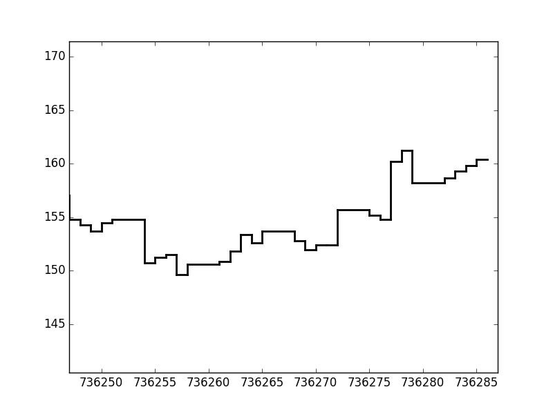
Fig 4 - Time-joined transformation of IBM stock
Figures 3 and 4 show the price path of IBM and its time-joined transformation, using the code above.
In this article, we have introduced the signature of a continuous path, as well as the signature of a stream of data. As we will see in the following articles, this object will prove to have very interesting applications to machine learning and time series analysis. After showing how to apply signatures to these fields, we will analyse concrete examples of how to use signatures in quantitative finance.
Article Series
- Rough Path Theory and Signatures Applied To Quantitative Finance - Part 1
- Rough Path Theory and Signatures Applied To Quantitative Finance - Part 2
- Rough Path Theory and Signatures Applied To Quantitative Finance - Part 3
- Rough Path Theory and Signatures Applied To Quantitative Finance - Part 4
References
- [1] Chevyrev, I., Kormilitzin, A. (2016) "A Primer on the Signature Method in Machine Learning, arXiv:1603.03788v1"
- [2] Gyurkó, G., Lyons, T., Kontkowski, M., Field J. (2013) "Extracting information from the signature of a financial data stream, arXiv:1307.7244"
- [3] Levin, D., Lyons, T., Ni, H. (2016) "Learning from the past, predicting the statistics for the future, learning an evolving system, 1309.0260"
- [4] Lyons, T., Ni, H., Oberhauser, H. (2014) "A feature set for streams and an application to high-frequency financial tick data.", Proceedings of the 2014 International Conference on Big Data Science and Computing, pg. 5
- [5] Lyons, T. (1998) "Differential equations driven by rough signals", Revista Matemática Iberoamericana 14 (2): 215-310