In a previous article the decision tree (DT) was introduced as a supervised learning method. In the article it was mentioned that the real power of DTs lies in their ability to perform extremely well as predictors when utilised in a statistical ensemble.
In this article it will be shown how combining multiple DTs in a statistical ensemble will vastly improve the predictive performance on the combined model. These statistical ensemble techniques are not limited to DTs, but are in fact applicable to many regression and classification machine learning models. However, DTs provide a "natural" setting to discuss ensemble methods and they are often commonly associated together.
Once the theory of these ensemble methods has been discussed they will all be implemented in Python using the Scikit-Learn library on financial data. In subsequent articles it will be shown how to apply such ensemble methods in real trading strategies using the QSTrader framework.
If you lack familiarity with decision trees it is worth reading the introductory article first before delving into ensemble methods.
Before discussing the ensemble techniques of bootstrap aggegration, random forests and boosting it is necessary to outline a technique from frequentist statistics known as the bootstrap, which enables these techniques to work.
The Bootstrap
Bootstrapping[1] is a statistical resampling technique that involves random sampling of a dataset with replacement. It is often used as a means of quantifying the uncertainty associated with a machine learning model.
For quantitative finance purposes bootstrapping is extremely useful since it allows generation of new samples from a population without having to go and collect additional "training data". In quantitative finance applications it is often impossible to generate more data in the case of financial asset pricing series as there is only one "history" to sample from.
The idea is to repeatedly sample data with replacement from the original training set in order to produce multiple separate training sets. These are then used to allow "meta-learner" or "ensemble" methods to reduce the variance of their predictions, thus greatly improving their predictive performance.
Two of the following ensemble techniques–bagging and random forests–make heavy use of bootstrapping techniques, and they will now be discussed.
Bootstrap Aggregation
As was mentioned in the article on decision tree theory one of the main drawbacks of DTs is that they suffer from being high-variance estimators. This means that the addition of a small number of extra training observations can dramatically alter the prediction performance of a learned tree, despite the training data not changing to any great extent.
This is in contrast to a low-variance estimator such as linear regression, which is not hugely sensitive to the addition of extra points–at least those that are relatively close to the remaining points.
One way to mitigate against this problem is to utilise a concept known as bootstrap aggregation or bagging. The idea is to combine multiple leaners (such as DTs), which are all fitted on separate bootstrapped samples and average their predictions in order to reduce the overall variance of these predictions.
Why does this work? James et al (2013)[2] point out that if $N$ independent and identically distributed (iid) observations $Z_1, \ldots, Z_N$ are given, each with a variance of $\sigma^2$ then the variance of the mean of the observations, $\bar{Z}$ is $\sigma^2 / N$. That is, if the average of these observations is taken the variance is reduced by factor equal to the number of observations.
However in quantitative finance datasets it is often the case that there is only one "training" set of data. This means it is difficult, if not impossible, to create multiple separate independent training sets. This is where The Bootstrap comes in, as it allows generation of multiple training sets all using one larger set.
Using the notation from James et al (2013)[2] and the Random Forest article at Wikipedia[3], if $B$ separate bootstrapped samples of the training set are created, with separate model estimators $\hat{f}^b ({\bf x})$, then averaging these leads to a low-variance estimator model, $\hat{f}_{\text{avg}}$:
\begin{eqnarray} \hat{f}_{\text{avg}} ({\bf x}) = \frac{1}{B} \sum^{B}_{b=1} \hat{f}^b ({\bf x}) \end{eqnarray}
This procedure is known as bagging[4]. It is highly applicable to DTs because they are high-variance estimators and this provides one mechanism to reduce the variance substantially.
Carrying out bagging for DTs is straightforward. Hundreds or thousands of deeply-grown (non-pruned) trees are created across $B$ bootstrapped samples of the training data. They are combined in the manner described above and significantly reduce the variance of the overall estimator.
One of the main benefits of bagging is that it is not possible to overfit the model solely by increasing the number of bootstrap samples, $B$. This is also true for random forests but not the method of boosting.
Unfortunately this gain in prediction accuracy comes at a price–significantly reduced interpretability of the model. However in quantitative trading research interpretability is often less important compared to raw prediction accuracy. Hence this is not too significant a drawback for algorithmic trading applications.
Note that there are specific statistical methods to deduce important variables in bagging, but they are beyond the scope of this article.
Random Forests
Random forests[5] are very similar to the procedure of bagging except that they make use of a technique called feature bagging, which has the advantage of significantly decreasing the correlation between each DT and thus increasing its predictive accuracy, on average.
Feature bagging works by randomly selecting a subset of the $p$ feature dimensions at each split in the growth of individual DTs. This may sound counterintuitive, after all it is often desired to include as many features as possible initially in order to gain as much information for the model. However it has the purpose of deliberately avoiding (on average) very strong predictive features that lead to similar splits in trees (and thus increase correlation).
That is, if a particular feature is strong in predicting the response value then it will be selected for many trees. Hence a standard bagging procedure can be quite correlated. Random forests avoid this by deliberately leaving out these strong features in many of the grown trees.
If all $p$ values are chosen in splitting of the trees in a random forest ensemble then this simply corresponds to standard bagging. A rule-of-thumb for random forests is to use $\sqrt{p}$ features, suitably rounded, at each split.
In the Python section below it will be shown how random forests compare to bagging in their performance as the number of DTs used as base estimators are increased.
Boosting
Another general machine learning ensemble method is known as boosting. Boosting differs somewhat from bagging as it does not involve bootstrap sampling. Instead models are generated sequentially and iteratively, meaning that it is necessary to have information about model $i$ before iteration $i+1$ is produced.
Boosting was motivated by Kearns and Valiant (1989)[6]. The question posed asked whether it was possible to combine, in some fashion, a selection of weak machine learning models to produce a single strong machine learning model. Weak, in this instance means a model that is only slightly better than chance at predicting a response. Correspondingly, a strong learner is one that is well-correlated to the true response.
This motivated the concept of boosting. The idea is to iteratively learn weak machine learning models on a continually-updated training data set and then add them together to produce a final, strong learning model. This differs from bagging, which simply averages the models on separate bootstrapped samples.
The basic algorithm for boosting, which is discussed at length in James et al (2013)[2] and Hastie et al (2009)[7], is given in the following:
- Set the initial estimator to zero, that is $\hat{f}({\bf x}) = 0$. Also set the residuals to the current responses, $r_i = y_i$, for all elements in the training set.
- Set the number of boosted trees, $B$. Loop over $b=1,\ldots,B$:
- Grow a tree $\hat{f}^b$ with $k$ splits to training data $(x_i, r_i)$, for all $i$.
- Add a scaled version of this tree to the final estimator: $\hat{f} ({\bf x}) \leftarrow \hat{f} ({\bf x}) + \lambda \hat{f}^b ({\bf x})$
- Update the residuals to account for the new model: $r_i \leftarrow r_i - \lambda \hat{f}^b (x_i)$
- Set the final boosted model to be the sum of individual weak learners: $\hat{f}({\bf x}) = \sum_{b=1}^B \lambda \hat{f}^b ({\bf x})$
Notice that each subsequent tree is fitted to the residuals of the data. Hence each subsequent iteration is slowly improving the overall strong learner by improving its performance in poorly-performing regions of the feature space.
It can be seen that this procedure is heavily dependent on the order in which the trees are grown. This process is said to "learn slowly". Such slow learning procedures tend to produce well-performing machine learning models. This is why ensemble algorithms involving boosted machine learning models tend to win many of the Kaggle competitions.
There are three hyperparameters to the boosting algorithm described above. Namely, the depth of the tree $k$, the number of boosted trees $B$ and the shrinkage rate $\lambda$. Some of these parameters can be set by cross-validation.
One of the computational drawbacks of boosting is that it is a sequential iterative method. This means that it cannot be easily parallelised, unlike bagging, which is straightforwardly parallelisable.
Many boosting algorithms exist, including AdaBoost, xgboost and LogitBoost. Prior to the increased prevalence of deep convolutional neural networks boosted trees often were (and still are!) some of the best "out of the box" classification tools in existence.
It will be shown how boosting compares with bagging, at least for the decision tree case, in the subsequent section.
Python Scikit-Learn Implementation
In this section the above three ensemble methods will be applied to the task of predicting the daily returns for Amazon stock, using the prior three days of lagged returns data.
This is a challenging task, not least because liquid stocks such as Amazon have a low signal-to-noise ratio, but also because such data is serially correlated. This means that the samples chosen are not truly independent of each other, which can have unfortunate consequences for the statistical validity of the procedure.
In subsequent articles a more robust procedure will be carried out using the Scikit-Learn time series cross-validation mechanism. For now, a standard training-testing split will be used, as the focus in this article is on comparison of error across the models and not on the absolute error achieved on each.
The end result will be a plot of the Mean Squared Error (MSE) of each method (bagging, random forest and boosting) against the number of estimators used in the sample. It will be clearly shown that bagging and random forests do not overfit as the number of estimators increases, while AdaBoost significantly overfits.
As always the first task is to import the correct libraries and objects. For this task many modules are required, the majority of which are in the Scikit-Learn library. In particular the "usual suspects" are imported, namely Matplotlib, NumPy, Pandas and Seaborn for data analysis and plotting. In addition the BaggingRegressor, RandomForestRegressor and AdaBoostRegressor ensemble methods are all included. Finally the mean_squared_error metric, the train_test_split cross-validation tool, preprocessing tool and DecisionTreeRegressor itself are all imported:
# ensemble_prediction.py

import datetime

import matplotlib.pyplot as plt
import numpy as np
import pandas as pd
import pandas_datareader.data as web
import seaborn as sns
import sklearn
from sklearn.ensemble import (
    BaggingRegressor, RandomForestRegressor, AdaBoostRegressor
)
from sklearn.metrics import mean_squared_error
from sklearn.model_selection import train_test_split
from sklearn.preprocessing import scale
from sklearn.tree import DecisionTreeRegressor
The next task is to use Pandas to create the DataFrame of lagged values. This particular piece of code has been utilised widely in Successful Algorithmic Trading and in other articles on the site. Hence it will not be explained in depth. The main thrust is that it creates a DataFrame containing three days of lagged returns data from a particular Yahoo Finance asset time series (as well as the daily trading volume):
def create_lagged_series(symbol, start_date, end_date, lags=3):
    """
    This creates a pandas DataFrame that stores
    the percentage returns of the adjusted closing
    value of a stock obtained from Yahoo Finance,
    along with a number of lagged returns from the
    prior trading days (lags defaults to 3 days).
    Trading volume is also included.
    """

    # Obtain stock information from Yahoo Finance
    ts = web.DataReader(
        symbol, "yahoo", start_date, end_date
    )

    # Create the new lagged DataFrame
    tslag = pd.DataFrame(index=ts.index)
    tslag["Today"] = ts["Adj Close"]
    tslag["Volume"] = ts["Volume"]

    # Create the shifted lag series of
    # prior trading period close values
    for i in range(0,lags):
        tslag["Lag%s" % str(i+1)] = ts["Adj Close"].shift(i+1)

    # Create the returns DataFrame
    tsret = pd.DataFrame(index=tslag.index)
    tsret["Volume"] = tslag["Volume"]
    tsret["Today"] = tslag["Today"].pct_change()*100.0

    # Create the lagged percentage returns columns
    for i in range(0,lags):
        tsret["Lag%s" % str(i+1)] = tslag[
            "Lag%s" % str(i+1)
        ].pct_change()*100.0
    tsret = tsret[tsret.index >= start_date]
    return tsret
In the __main__ function the parameters are set. Firstly a random seed is defined to make the code replicable on other work environments. n_jobs controls the number of processor cores to use in bagging and random forests. Boosting is not parallelisable so does not make use of this parameter.
n_estimators defines the total number of estimators to use in the graph of the MSE, while the step_factor controls how granular the calculation is by stepping through the number of estimators. In this instance axis_step is equal to 1000/10 = 100. That is, 100 separate calculations will be performed for each of the three ensemble methods:
# Set the random seed, number of estimators
# and the "step factor" used to plot the graph of MSE
# for each method
random_state = 42
n_jobs = 1  # Parallelisation factor for bagging, random forests
n_estimators = 1000
step_factor = 10
axis_step = int(n_estimators/step_factor)
The following code downloads ten years worth of AMZN prices and converts them into a return series with lags using the above mentioned function create_lagged_series. Missing values are dropped (a consequence of the lag procedure) and the data is scaled to exist between -1 and +1 for ease of comparison. This latter procedure is common in machine learning and helps features with large differences in absolute sizes be comparable to the models:
# Download ten years worth of Amazon
# adjusted closing prices
start = datetime.datetime(2006, 1, 1)
end = datetime.datetime(2015, 12, 31)
amzn = create_lagged_series("AMZN", start, end, lags=3)
amzn.dropna(inplace=True)

# Use the first three daily lags of AMZN closing prices
# and scale the data to lie within -1 and +1 for comparison
X = amzn[["Lag1", "Lag2", "Lag3"]]
y = amzn["Today"]
X = scale(X)
y = scale(y)
The data is split into a training set and a test set, with 70% of the data forming the training data and the remaining 30% performing the test set. Once again, be aware that financial time series data is serially correlated and so this procedure will introduce some error by not accounting for it. However it serves the purpose for comparison across procedures in this article:
# Use the training-testing split with 70% of data in the
# training data with the remaining 30% of data in the testing
X_train, X_test, y_train, y_test = train_test_split(
    X, y, test_size=0.3, random_state=random_state
)
The following NumPy arrays store the number of estimators at each axis step, as well as the actual associated MSE for each of the three ensemble methods. They are all initially set to zero and are filled in subsequently:
# Pre-create the arrays which will contain the MSE for
# each particular ensemble method
estimators = np.zeros(axis_step)
bagging_mse = np.zeros(axis_step)
rf_mse = np.zeros(axis_step)
boosting_mse = np.zeros(axis_step)
The first ensemble method to be utilised is the bagging procedure. The code iterates over the total number of estimators (1 to 1000 in this case, with a step-size of 10), defines the ensemble model with the correct base model (in this case a regression decision tree), fits it to the training data and then calculates the Mean Squared Error on the test data. This MSE is then added to the bagging MSE array:
# Estimate the Bagging MSE over the full number
# of estimators, across a step size ("step_factor")
for i in range(0, axis_step):
    print("Bagging Estimator: %d of %d..." % (
        step_factor*(i+1), n_estimators)
    )
    bagging = BaggingRegressor(
        DecisionTreeRegressor(),
        n_estimators=step_factor*(i+1),
        n_jobs=n_jobs,
        random_state=random_state
    )
    bagging.fit(X_train, y_train)
    mse = mean_squared_error(y_test, bagging.predict(X_test))
    estimators[i] = step_factor*(i+1)
    bagging_mse[i] = mse
The same approach is carried out for random forests. Since random forests implicitly use a regression tree as their base estimators there is no need to specify it in the ensemble constructor:
# Estimate the Random Forest MSE over the full number
# of estimators, across a step size ("step_factor")
for i in range(0, axis_step):
    print("Random Forest Estimator: %d of %d..." % (
        step_factor*(i+1), n_estimators)
    )
    rf = RandomForestRegressor(
        n_estimators=step_factor*(i+1),
        n_jobs=n_jobs,
        random_state=random_state
    )
    rf.fit(X_train, y_train)
    mse = mean_squared_error(y_test, rf.predict(X_test))
    estimators[i] = step_factor*(i+1)
    rf_mse[i] = mse
Similarly for the AdaBoost boosting algorithm although n_jobs is not present due to the lack of parallelisability of boosting techniques. The learning rate, or shrinkage factor, $\lambda$ has been set to 0.01. Adjusting this value has a large impact on the absolute MSE calculated for each estimator total:
# Estimate the AdaBoost MSE over the full number
# of estimators, across a step size ("step_factor")
for i in range(0, axis_step):
    print("Boosting Estimator: %d of %d..." % (
        step_factor*(i+1), n_estimators)
    )
    boosting = AdaBoostRegressor(
        DecisionTreeRegressor(),
        n_estimators=step_factor*(i+1),
        random_state=random_state,
        learning_rate=0.01
    )
    boosting.fit(X_train, y_train)
    mse = mean_squared_error(y_test, boosting.predict(X_test))
    estimators[i] = step_factor*(i+1)
    boosting_mse[i] = mse
The final snippet of code simply plots these arrays against each other using Matplotlib, but with Seaborn's default colour scheme, which is more visually pleasing than the Matplotlib defaults:
# Plot the chart of MSE versus number of estimators
plt.figure(figsize=(8, 8))
plt.title('Bagging, Random Forest and Boosting comparison')
plt.plot(estimators, bagging_mse, 'b-', color="black", label='Bagging')
plt.plot(estimators, rf_mse, 'b-', color="blue", label='Random Forest')
plt.plot(estimators, boosting_mse, 'b-', color="red", label='AdaBoost')
plt.legend(loc='upper right')
plt.xlabel('Estimators')
plt.ylabel('Mean Squared Error')
plt.show()
The output is given in the following figure. It is very clear how increasing the number of estimators for the bootstrap-based methods (bagging and random forests) eventually leads to the MSE "settling down" and becoming almost identical between them. However, for the AdaBoost boosting algorithm it can be seen that as the number of estimators is increased beyond 100 or so, the method begins to significantly overfit.
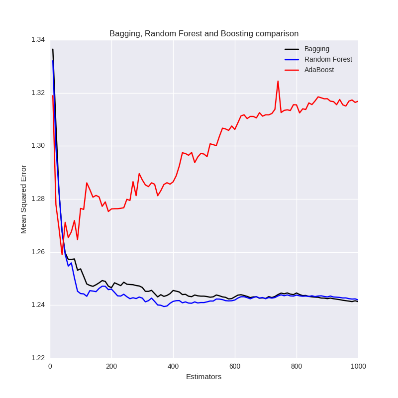 Bagging, Random Forest and AdaBoost MSE comparison vs number of estimators in the ensemble
When constructing a trading strategy based on a boosting ensemble procedure this fact must be borne in mind otherwise it is likely to lead to significant underperformance of the strategy when applied to out-of-sample financial data.
In a subsequent article ensemble models will be utilised to predict asset returns using QSTrader. It will be seen whether it is feasible to produce a robust strategy that can be profitable above the higher frequency transaction costs necessary to carry it out.
References
- [1] Efron, B. (1979) "Bootstrap methods: Another look at the jackknife", The Annals of Statistics 7 (1): 1-26
- [2] James, G., Witten, D., Hastie, T., Tibshirani, R. (2013) An Introduction to Statistical Learning, Springer
- [3] Wikipedia (2016) Wikipedia: Random Forest, https://en.wikipedia.org/wiki/Random_forest
- [4] Breiman, L. (1996) "Bagging predictors", Machine Learning 24 (2): 123-140
- [5] Breiman, L. (2001) "Random Forests", Machine Learning 45 (1): 5-32
- [6] Kearns, M., Valiant, L. (1989) "Crytographic limitations on learning Boolean formulae and finite automata", Symposium on Theory of computing. ACM. 21 (None): 433-444
- [7] Hastie, T., Tibshirani, R., Friedman, J. (2009) The Elements of Statistical Learning, Springer
Full Code
# ensemble_prediction.py

import datetime

import matplotlib.pyplot as plt
import numpy as np
import pandas as pd
import pandas_datareader.data as web
import seaborn as sns
import sklearn
from sklearn.ensemble import (
    BaggingRegressor, RandomForestRegressor, AdaBoostRegressor
)
from sklearn.metrics import mean_squared_error
from sklearn.model_selection import train_test_split
from sklearn.preprocessing import scale
from sklearn.tree import DecisionTreeRegressor


def create_lagged_series(symbol, start_date, end_date, lags=3):
    """
    This creates a pandas DataFrame that stores
    the percentage returns of the adjusted closing
    value of a stock obtained from Yahoo Finance,
    along with a number of lagged returns from the
    prior trading days (lags defaults to 3 days).
    Trading volume is also included.
    """

    # Obtain stock information from Yahoo Finance
    ts = web.DataReader(
        symbol, "yahoo", start_date, end_date
    )

    # Create the new lagged DataFrame
    tslag = pd.DataFrame(index=ts.index)
    tslag["Today"] = ts["Adj Close"]
    tslag["Volume"] = ts["Volume"]

    # Create the shifted lag series of
    # prior trading period close values
    for i in range(0,lags):
        tslag["Lag%s" % str(i+1)] = ts["Adj Close"].shift(i+1)

    # Create the returns DataFrame
    tsret = pd.DataFrame(index=tslag.index)
    tsret["Volume"] = tslag["Volume"]
    tsret["Today"] = tslag["Today"].pct_change()*100.0

    # Create the lagged percentage returns columns
    for i in range(0,lags):
        tsret["Lag%s" % str(i+1)] = tslag[
            "Lag%s" % str(i+1)
        ].pct_change()*100.0
    tsret = tsret[tsret.index >= start_date]
    return tsret


if __name__ == "__main__":
    # Set the random seed, number of estimators
    # and the "step factor" used to plot the graph of MSE
    # for each method
    random_state = 42
    n_jobs = 1  # Parallelisation factor for bagging, random forests
    n_estimators = 1000
    step_factor = 10
    axis_step = int(n_estimators/step_factor)

    # Download ten years worth of Amazon
    # adjusted closing prices
    start = datetime.datetime(2006, 1, 1)
    end = datetime.datetime(2015, 12, 31)
    amzn = create_lagged_series("AMZN", start, end, lags=3)
    amzn.dropna(inplace=True)

    # Use the first three daily lags of AMZN closing prices
    # and scale the data to lie within -1 and +1 for comparison
    X = amzn[["Lag1", "Lag2", "Lag3"]]
    y = amzn["Today"]
    X = scale(X)
    y = scale(y)

    # Use the training-testing split with 70% of data in the
    # training data with the remaining 30% of data in the testing
    X_train, X_test, y_train, y_test = train_test_split(
        X, y, test_size=0.3, random_state=random_state
    )

    # Pre-create the arrays which will contain the MSE for
    # each particular ensemble method
    estimators = np.zeros(axis_step)
    bagging_mse = np.zeros(axis_step)
    rf_mse = np.zeros(axis_step)
    boosting_mse = np.zeros(axis_step)

    # Estimate the Bagging MSE over the full number
    # of estimators, across a step size ("step_factor")
    for i in range(0, axis_step):
        print("Bagging Estimator: %d of %d..." % (
            step_factor*(i+1), n_estimators)
        )
        bagging = BaggingRegressor(
            DecisionTreeRegressor(),
            n_estimators=step_factor*(i+1),
            n_jobs=n_jobs,
            random_state=random_state
        )
        bagging.fit(X_train, y_train)
        mse = mean_squared_error(y_test, bagging.predict(X_test))
        estimators[i] = step_factor*(i+1)
        bagging_mse[i] = mse

    # Estimate the Random Forest MSE over the full number
    # of estimators, across a step size ("step_factor")
    for i in range(0, axis_step):
        print("Random Forest Estimator: %d of %d..." % (
            step_factor*(i+1), n_estimators)
        )
        rf = RandomForestRegressor(
            n_estimators=step_factor*(i+1),
            n_jobs=n_jobs,
            random_state=random_state
        )
        rf.fit(X_train, y_train)
        mse = mean_squared_error(y_test, rf.predict(X_test))
        estimators[i] = step_factor*(i+1)
        rf_mse[i] = mse

    # Estimate the AdaBoost MSE over the full number
    # of estimators, across a step size ("step_factor")
    for i in range(0, axis_step):
        print("Boosting Estimator: %d of %d..." % (
            step_factor*(i+1), n_estimators)
        )
        boosting = AdaBoostRegressor(
            DecisionTreeRegressor(),
            n_estimators=step_factor*(i+1),
            random_state=random_state,
            learning_rate=0.01
        )
        boosting.fit(X_train, y_train)
        mse = mean_squared_error(y_test, boosting.predict(X_test))
        estimators[i] = step_factor*(i+1)
        boosting_mse[i] = mse

    # Plot the chart of MSE versus number of estimators
    plt.figure(figsize=(8, 8))
    plt.title('Bagging, Random Forest and Boosting comparison')
    plt.plot(estimators, bagging_mse, 'b-', color="black", label='Bagging')
    plt.plot(estimators, rf_mse, 'b-', color="blue", label='Random Forest')
    plt.plot(estimators, boosting_mse, 'b-', color="red", label='AdaBoost')
    plt.legend(loc='upper right')
    plt.xlabel('Estimators')
    plt.ylabel('Mean Squared Error')
    plt.show()


