In the recent previous article on Correlation Matrix Generation using Object Oriented Python we created a Python object-oriented class hierarchy to develop an extensible, modular tool for generating synthetic correlation matrices. Such matrices can be used to generated synthetic correlated time series models, which can form the basis of realistic synthetic financial datasets.
In this article we are going to continue the development of the synthetic dataset generating tool by developing another object-oriented class hierarchy for the time series generator model components. These will form the basis of correlated synthetic asset pricing data.
We will consider two models—namely the Geometric Brownian Motion (GBM) and Jump-Diffusion (JD) stochastic process models—and demonstrate how they can both be implemented via this class hierarchy.
Once we have implemented both models we will code up a Matplotlib-based visualisation script. We will use it to compare each of the models' behaviours side by side for a number of path realisations.
Here is a sneak preview of the output of the tools we will develop in this article:
We will begin by developing the abstract base class that defines the time series model class interface. Then we will implement both the GBM and JD derived subclasses. Then we will use these classes to generate some sample paths.
Abstract Base Class
The first task is to define the class interface, in a similar manner to the previous article. This will require importing the appropriate Python ABC machinery and the third party NumPy library, which will be used to store the price paths. This will be stored in a new file called models.py:
# models.py

from abc import ABC, abstractmethod
from typing import Tuple, Optional

import numpy as np
The next task is to create a TimeSeriesModel base class that will define the interface for all subsequent time series model derived subclasses.
The __init__ initialisation method takes in two arguments--the starting price $S_0$, start_price, and the time series model time step $\Delta t$, dt. The latter defaults to $1/252$, which accounts for the approximately 252 business days per year (since we are currently considering daily pricing models):
# ..
# models.py
# ..

class TimeSeriesModel(ABC):
    """
    Abstract base class for time series models.
    """

    def __init__(
        self,
        start_price: float,
        dt: float = 1/252
    ):
        """
        Initialize the time series model.

        Args:
            start_price: Initial price of the asset
            dt: Time step (default: 1/252 for daily data)
        """
        self.start_price = start_price
        self.dt = dt
The class interface exposes a single "public" method generate_path. This method takes in a number of steps n (essentially days to generate pricing for) and a NumPy array of random variable sample draws called random_shocks. The latter provides the correlated random variables that will be used to correlate multiple separate realisations of the time series models together. The method is designed to return a NumPy array containing the prices of a single realisation of the model:
# ..
# models.py
# ..

    @abstractmethod
    def generate_path(
        self,
        n_steps: int,
        random_shocks: np.ndarray
    ) -> np.ndarray:
        """
        Generate a price path given random shocks.

        Args:
            n_steps: Number of time steps
            random_shocks: Array of random shocks (already correlated)

        Returns:
            Array of prices
        """
        pass
Now that we have developed the class interface for these time series we can discuss the actual concrete implementations, beginning with Geometric Brownian Motion.
Geometric Brownian Motion
We have discussed Geometric Brownian Motion extensively on QuantStart (see the previous articles on Geometric Brownian Motion and Geometric Brownian Motion Simulation with Python), but we are going to provide a mathematical recap in the information box below, to help refamiliarise you with the concept if you haven't seen the mathematical details in a while.
Geometric Brownian is a very common Stochastic Differential Equation (SDE) model for the time-evolution of an asset price $S(t)$. The SDE for GBM is given by:
\begin{eqnarray} dS(t) = \mu S(t) dt + \sigma S(t) dB(t) \end{eqnarray}Note that the coefficients $\mu$ and $\sigma$, representing the drift and volatility of the asset, respectively, are both constant in this model. In more sophisticated models they can be made to be functions of $t$, $S(t)$ and other stochastic processes (such as with Stochastic Volality models).
The solution $S(t)$ can be found by the application of Ito's Lemma to the stochastic differential equation. We won't derive this in full here, but will simply present the result:
\begin{eqnarray} S(t) = S(0) \exp \left(\left(\mu - \frac{1}{2}\sigma^2\right)t + \sigma B(t)\right) \end{eqnarray}We will now use this formulae, along with an appropriate numerical method such as the Euler-Maruyama discretisation, to develop a Python code to simulate single realisations of this model.
To implement the Geometric Brownian Motion model we first code up the __init__ initialization method. We provide the two arguments that formed the interface for the base TimeSeriesModel class, namely start_price and dt. We also provide two additional floating point valued keyword arguments drift and volatility, which are used to parameterize the model behaviour:
# ..
# models.py
# ..

class GeometricBrownianMotion(TimeSeriesModel):
    """
    Geometric Brownian Motion model for asset prices.
    """

    def __init__(
        self,
        start_price: float,
        dt: float,
        drift: float = 0.0,
        volatility: float = 0.2,
    ):
        """
        Initialize the Geometric Brownian Motion model.

        Args:
            start_price: Initial price of the asset
            dt: Time step (default: 1/252 for daily data)
            drift: Annual drift parameter (mu)
            volatility: Annual volatility parameter (sigma)
        """
        super().__init__(start_price, dt)
        self.drift = drift
        self.volatility = volatility
The next step is to code up the generate_path method. As previously mentioned this requires two arguments, n for the number of steps in the path and random_shocks, which is used for receiving the correlated random variables from an external controlling class that will be developed in subsequent articles.
The method initially creates a one-dimensional (1D) prices array and sets the first value equal to the provided starting price. We then precalculate the value of $\sqrt{\Delta t}$ to avoid calculating this unnecessarily within the loop.
We now iterate over the number of steps and calculate both the drift and diffusion components of GBM. Importantly, note the usage of random_shocks within the diffusion term. Finally, the next price instance $S(t+1)$ is calculated as the multiple of the current price $S(0)$ and the exponential of the sum of the drift and the diffusion components.
We do not need to return the first price in the array as this will be calculated by an external class:
# ..
# models.py
# ..

    def generate_path(
        self,
        n_steps: int,
        random_shocks: np.ndarray
    ) -> np.ndarray:
        """
        Generate a GBM price path.
        """
        prices = np.zeros(n_steps + 1)
        prices[0] = self.start_price

        # GBM formula: S(t+dt) = S(t) * exp((mu - 0.5*sigma^2)*dt + sigma*sqrt(dt)*Z)
        dt_sqrt = np.sqrt(self.dt)

        for t in range(n_steps):
            drift_component = (self.drift - 0.5 * self.volatility**2) * self.dt
            diffusion_component = self.volatility * dt_sqrt * random_shocks[t]
            prices[t + 1] = prices[t] * np.exp(drift_component + diffusion_component)

        return prices[1:]  # Return prices excluding the initial price
This completes the implementation of the GeometricBrownianMotion stochastic process model. While this model is a useful starting point for modelling equities behaviour (and is used within many options pricing tools), it does not include a number of "stylised facts" that are present in real equities pricing series.
This includes volatility clustering behaviour, as well as random jumps (e.g. due to significant price-affecting news occuring overnight). The latter effects can be modelled by the so-called Jump-Diffusion model, which will be implemented in the next section.
Jump Diffusion
The following code snippets implement the JumpDiffusion time series model, which includes stochastic price jumps to model the effects of information that can dramatically and rapidly alter the stock price of a company. The model is essentially a Geometric Brownian Motion path (with all of the associated parameters) that is periodically subjected to Poisson model distributed stochastic jumps of a certain magnitude (the magnitudes are also stochastic).
For the initialization method __init__ we add three new parameters compared to Geomtric Brownian Motion. The first is jump_intensity, which measures the average number of jumps per year ($\lambda$). The second is jump_mean, which is the mean average value of the jump. The final value is jump_std, which measures the standard deviation of the jump magnitude:
# ..
# models.py
# ..

class JumpDiffusion(TimeSeriesModel):
    """
    Jump-Diffusion model for asset prices.
    """

    def __init__(
        self,
        start_price: float,
        dt: float = 1/252,
        drift: float = 0.0,
        volatility: float = 0.2,
        jump_intensity: float = 0.1,
        jump_mean: float = 0.0,
        jump_std: float = 0.1,
    ):
        """
        Initialize the Jump-Diffusion model.

        Args:
            start_price: Initial price of the asset
            dt: Time step (default: 1/252 for daily data)
            drift: Annual drift parameter (mu)
            volatility: Annual volatility parameter (sigma)
            jump_intensity: Average number of jumps per year (lambda)
            jump_mean: Mean of jump size (log-normal)
            jump_std: Standard deviation of jump size (log-normal)
        """
        super().__init__(start_price, dt)
        self.drift = drift
        self.volatility = volatility
        self.jump_intensity = jump_intensity
        self.jump_mean = jump_mean
        self.jump_std = jump_std
As the following generate_path method includes some fairly complex probability and statistics assumptions regarding the modelling of jumps, we have included a full info box to describe the assumptions that go into the model. If you are familiar with how Jump-Diffusion models work then you can skip this and jump straight to the code below.
The generate_path method implements the Jump-Diffusion model, which combines continuous Geometric Brownian Motion with discontinuous Poisson-distributed jumps. In our implementation below we actually utilise binomial distributions to represent Poisson jumps. This is because when $\Delta t$ (dt) is small (as it typically is for daily time steps like $\Delta t = 1/252$), the probability of multiple jumps occurring in a single time step becomes negligible.
In this limit, a Poisson process with rate $\lambda \Delta t$ can be well-approximated by a Bernoulli (binomial with $n=1$) random variable that takes value 1 with probability $\lambda \Delta t$ and 0 otherwise. This is why the code uses np.random.binomial(1, jump_probs, n_steps) where jump_probs = self.jump_intensity * self.dt. It is determining whether a jump occurs (1) or not (0) at each time step.
The method then generates jump sizes only for time steps where jumps occur. These jump sizes follow a log-normal distribution (controlled by jump_mean and jump_std), which ensures that prices remain positive after jumps. The expression np.exp(np.random.normal(...)) - 1 converts the log-normal random variable into a returns (rather than price) format - if $J$ is log-normal, then $(J - 1)$ represents the proportional change in price. The continuous component follows standard GBM dynamics with the drift and diffusion terms, where the drift includes the usual Itô correction term (-0.5 * volatility^2).
Finally, the price evolution combines both components multiplicatively: prices[t + 1] = prices[t] * np.exp(drift_component + diffusion_component) * (1 + jump_component). The GBM part is applied as an exponential (ensuring positive prices), while the jump is applied as a multiplicative factor (1 + jump_component).
This formulation ensures that jumps create proportional changes in price rather than absolute changes, which is more realistic for financial assets. The usefulness of this approximation is that it's both computationally efficient and mathematically sound for typical financial modeling time scales, avoiding the need to explicitly sample from a Poisson distribution and handle the rare cases of multiple jumps per time step.
The code begins by generating a zero array prices, for which the first value is filled with the starting price. As with the GBM implementation, we precalculate $\sqrt{\Delta t}$. Subsequently the probabilities and actual occurence dates for the jumps are calculated using the approach outlined in the info box describing the model. The number of jumps is then calculated as the sum of the occurences of jumps (since each entry in jumps_occur is unity).
If there is a non-zero number of jumps, each of the one-valued entries of the jump_sizes array is set to a stochastic log-normal jump value. The remainder of the method is similar to the implementation for Geometric Brownian Motion, with the exception of multiplying the prices by 1 + jump_component to take into account multiplicative (proportional) jumps:
# ..
# models.py
# ..

    def generate_path(
        self,
        n_steps: int,
        random_shocks: np.ndarray
    ) -> np.ndarray:
        """
        Generate a Jump-Diffusion price path.
        """
        prices = np.zeros(n_steps + 1)
        prices[0] = self.start_price

        dt_sqrt = np.sqrt(self.dt)

        # Generate jump occurrences
        jump_probs = self.jump_intensity * self.dt
        jumps_occur = np.random.binomial(1, jump_probs, n_steps)

        # Generate jump sizes
        jump_sizes = np.zeros(n_steps)
        n_jumps = jumps_occur.sum()
        if n_jumps > 0:
            # Log-normal jumps
            jump_sizes[jumps_occur == 1] = np.exp(
                np.random.normal(self.jump_mean, self.jump_std, n_jumps)
            ) - 1

        for t in range(n_steps):
            # GBM component
            drift_component = (self.drift - 0.5 * self.volatility**2) * self.dt
            diffusion_component = self.volatility * dt_sqrt * random_shocks[t]

            # Jump component
            jump_component = jump_sizes[t]

            # Combined price evolution
            prices[t + 1] = prices[t] * np.exp(drift_component + diffusion_component) * (1 + jump_component)

        return prices[1:]  # Return prices excluding the initial price
This completes models.py. As with the correlation.py module described in the previous article, this module has no entrypoint and solely contains the class definitions and implementations for the time series models. We are now going to use a similar approach to the previous article which visualised the correlation matrix instances. This will involve visualising a set of paths drawn from each of the respective Geometric Brownian Motion and Jump-Diffusion models.
To achieve this we will write a short visualization script that will display a selection of random sample paths from each of the time series models side-by-side, within the next section.
Asset Price Path Visualization
We can utilise NumPy and Matplotlib to create the visualisations of each of the respective time series models' samples. We create a new file called models_visualization.py and place it in the same directory as models.py. We can utilise Matplotlib's plot method to plot the trading day index against the asset price path value(s), for each respective model.
We first import the necessary libraries and the classes we have just implemented from models.py:
# models_visualization.py

import matplotlib.pyplot as plt
import numpy as np

from models import (
    GeometricBrownianMotion,
    JumpDiffusion
)
The first function to implement is generate_paths. It takes in a number of parameters. The first is the time series model instance model, which for this example will either be the Geometric Brownian Motion or Jump-Diffusion class model instance. It requires the number of steps, n_steps, which defaults to 252 (one year) for this example. It also requires the number of separate path realizations to plot, n_paths. Finally, it is possible to provide an optional random seed to ensure you can reproduce the results, via seed.
This function initially sets the random seed, if provided. Then it creates an empty two-dimensional matrix of zeros of size (n_paths, n_steps) to store the eventual path realisation values. Then it loops over each path and generates the 'random shocks' array, that store the random variables used in each of the models. In later articles we will not simply use standard Normal (Gaussian) values here, instead we will values that provide correlations across each path instance via a technique known as Cholesky Decomposition.
Finally, we create each of the paths themselves by calling each model's respective generate_paths method with the number of required steps and the random_shocks array of random variables:
# ..
# models_visualization.py
# ..

def generate_paths(model, n_steps, n_paths, seed=None):
    """
    Generate multiple price paths for a given model.

    Args:
        model: TimeSeriesModel instance
        n_steps: Number of time steps per path
        n_paths: Number of paths to generate
        seed: Random seed for reproducibility

    Returns:
        Array of shape (n_paths, n_steps) containing all price paths
    """
    if seed is not None:
        np.random.seed(seed)

    paths = np.zeros((n_paths, n_steps))

    for i in range(n_paths):
        # Generate uncorrelated standard normal shocks
        random_shocks = np.random.standard_normal(n_steps)
        paths[i] = model.generate_path(n_steps, random_shocks)

    return paths
The next function to implement is plot_model_paths. This function takes in multiple parameters. Firstly, it requires a Matplotlib Axes object on which to produce the plots. It requires the (n_paths, n_steps)-sized 2D NumPy array that was generated in the previous function, called paths. It then requires the name of the time series model used (model_name) to name the model in the figure. It requires $\Delta t$ (dt) in order to calculate the correct number of time steps utilised. Finally, it takes in alpha transparency value (alpha) to add to the path plot lines.
The function iterates over the number of paths and uses the Matplotlib line plot plot method to plot the calculated time steps (time_steps) against the individual path row stores in the 2D paths array, with the given alpha transparency and a pre-set line width.
It also adds the mean average path, calculated across all path realisations provided, in a stronger black color to emphasise the sample average behaviour of the model. Finally, some x- and y-axis labels are added, along with a title, a grid and a legend:
# ..
# models_visualization.py
# ..

def plot_model_paths(ax, paths, model_name, dt, alpha=0.3):
    """
    Plot multiple paths on a given axes.

    Args:
        ax: Matplotlib axes object
        paths: Array of shape (n_paths, n_steps) containing price paths
        model_name: Name of the model for the title
        dt: Time step size
        alpha: Transparency level for the paths
    """
    n_paths, n_steps = paths.shape
    time_steps = np.arange(n_steps) * dt * 252  # Convert to trading days

    # Plot all paths with transparency
    for i in range(n_paths):
        ax.plot(time_steps, paths[i], alpha=alpha, linewidth=0.8)

    # Calculate and plot mean path in bold
    mean_path = np.mean(paths, axis=0)
    ax.plot(time_steps, mean_path, 'k-', linewidth=2, label='Mean', alpha=0.8)

    ax.set_xlabel('Time (trading days)')
    ax.set_ylabel('Price')
    ax.set_title(f'{model_name} - {n_paths} Path Realizations')
    ax.grid(True, alpha=0.8)
    ax.legend(loc='best')
With these two functions created it is now possible to implement the entrypoint with the main function.
The first section of this entrypoint sets a number of parameters, including the number of paths, the number of time steps, the starting price of the models, the daily time step, the respective models' drifts and volatilities, as well as model specific parameters and finally a random seed for reproducibility. Each of the parameters is commented to highlight how they relate to the previous model implementations:
# ..
# models_visualization.py
# ..

def main():
    # Configuration parameters
    k = 50  # Number of path realizations
    n_steps = 252  # Number of time steps (1 year of daily data)

    # Model parameters
    start_price = 100.0
    dt = 1/252  # Daily time step

    # GBM parameters
    gbm_drift = 0.05  # 5% annual drift
    gbm_volatility = 0.2  # 20% annual volatility

    # Jump-Diffusion parameters
    jd_drift = 0.05  # 5% annual drift
    jd_volatility = 0.15  # 15% annual volatility (lower than GBM since jumps add volatility)
    jump_intensity = 5.0  # Average 5 jumps per year
    jump_mean = -0.03  # Average jump size (log-normal mean)
    jump_std = 0.06  # Jump size standard deviation

    # Random seed for reproducibility (set to None for random results)
    seed = 42
In the next section of the main function a Geometric Brownian Motion model gbm_model and a Jump-Diffusion model jd_model are both instantiated with all of the previous parameters defined above:
# ..
# models_visualization.py
# ..

    # Initialize models
    gbm_model = GeometricBrownianMotion(
        start_price=start_price,
        dt=dt,
        drift=gbm_drift,
        volatility=gbm_volatility
    )

    jd_model = JumpDiffusion(
        start_price=start_price,
        dt=dt,
        drift=jd_drift,
        volatility=jd_volatility,
        jump_intensity=jump_intensity,
        jump_mean=jump_mean,
        jump_std=jump_std
    )
The final section of the main function generates the various path realisations from each model using the respective generate_paths method. Then a Matplotlib subplots figure is created, with one row and two columns. Each of the models' paths are plotted on a separate axis object using the model instances defined previously.
Finally, a title is aadded and the figure is shown to the screen (or optionally persisted to disk as a PNG):
# ..
# models_visualization.py
# ..

    # Generate paths
    print("\nGenerating paths...")
    gbm_paths = generate_paths(gbm_model, n_steps, k, seed=seed)
    jd_paths = generate_paths(jd_model, n_steps, k, seed=seed if seed else None)

    # Create figure with two subplots
    fig, (ax1, ax2) = plt.subplots(1, 2, figsize=(15, 6))

    # Plot GBM paths
    plot_model_paths(ax1, gbm_paths, "Geometric Brownian Motion", dt, alpha=0.5)

    # Plot Jump-Diffusion paths
    plot_model_paths(ax2, jd_paths, "Jump-Diffusion", dt, alpha=0.5)

    # Add overall title
    fig.suptitle('Comparison of Time Series Models', fontsize=16)

    # Adjust layout
    plt.tight_layout()

    # Display the plot
    plt.show()

    # Optional: Save the figure
    # plt.savefig('asset_price_path_visualization.png', dpi=150, bbox_inches='tight')
Finally, in order to ensure the correct function is run when the file is called with Python from the command line it is necessary to call the main function in the entrypoint:
# ..
# models_visualization.py
# ..

if __name__ == "__main__":
    main()
In a suitable virtual environment you can run the following command in the terminal:
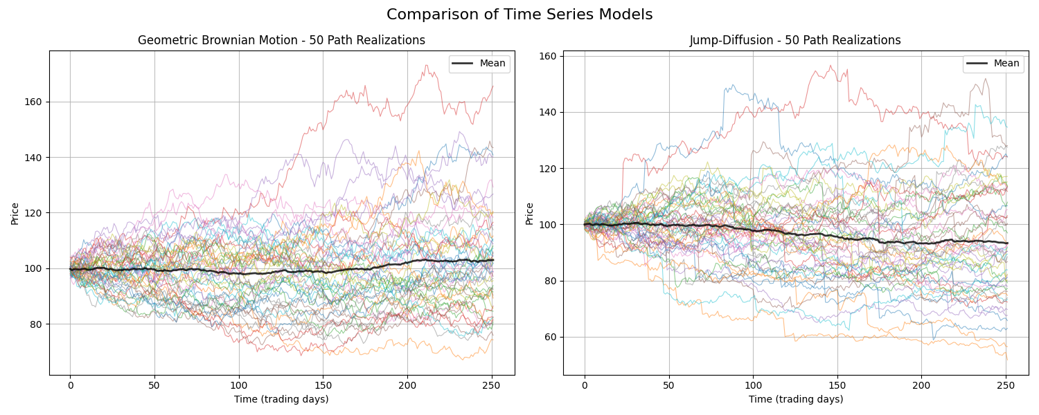
python3 models_visualization.pyThe results of this script can be seen in the figure below. The left hand side displays a selection of 50 sample paths from the Geometric Brownian Motion model, along with the black sample mean average path. The right hand side displays a selection of 50 sample paths from the Jump-Diffusion model, along with another black sample mean average path.
The number of jumps along with the jump scale has been chosen specifically here to emphasis the differences in the two models. It is clear that the Jump-Diffusion paths contain a number of distinct sharp upward/downward jumps in pricing throughout the path history. As the jump mean was chosen to be slightly negative, it can be seen that this overcomes the slight upward drift to produce a decreasing sample mean average path.
Next Steps
We have now developed two of the components for our synthetic data generation tool with the correlation matrix generator and the time series model class hierarchies. In the next article we are going to develop the component that will generate the correlated random variables using a technique known as Cholesky Decomposition, which will be used to generate correlated price paths. We will then demonstrate how these paths can be persisted to disk in a CSV format, useable in downstream systematic trading systems.
Full Code
# models.py

from abc import ABC, abstractmethod
from typing import Tuple, Optional

import numpy as np


class TimeSeriesModel(ABC):
    """
    Abstract base class for time series models.
    """

    def __init__(
        self,
        start_price: float,
        dt: float = 1/252
    ):
        """
        Initialize the time series model.

        Args:
            start_price: Initial price of the asset
            dt: Time step (default: 1/252 for daily data)
        """
        self.start_price = start_price
        self.dt = dt

    @abstractmethod
    def generate_path(
        self,
        n_steps: int,
        random_shocks: np.ndarray
    ) -> np.ndarray:
        """
        Generate a price path given random shocks.

        Args:
            n_steps: Number of time steps
            random_shocks: Array of random shocks (already correlated)

        Returns:
            Array of prices
        """
        pass


class GeometricBrownianMotion(TimeSeriesModel):
    """
    Geometric Brownian Motion model for asset prices.
    """

    def __init__(
        self,
        start_price: float,
        dt: float,
        drift: float = 0.0,
        volatility: float = 0.2,
    ):
        """
        Initialize the Geometric Brownian Motion model.

        Args:
            start_price: Initial price of the asset
            dt: Time step (default: 1/252 for daily data)
            drift: Annual drift parameter (mu)
            volatility: Annual volatility parameter (sigma)
        """
        super().__init__(start_price, dt)
        self.drift = drift
        self.volatility = volatility

    def generate_path(
        self,
        n_steps: int,
        random_shocks: np.ndarray
    ) -> np.ndarray:
        """
        Generate a GBM price path.
        """
        prices = np.zeros(n_steps + 1)
        prices[0] = self.start_price

        # GBM formula: S(t+dt) = S(t) * exp((mu - 0.5*sigma^2)*dt + sigma*sqrt(dt)*Z)
        dt_sqrt = np.sqrt(self.dt)

        for t in range(n_steps):
            drift_component = (self.drift - 0.5 * self.volatility**2) * self.dt
            diffusion_component = self.volatility * dt_sqrt * random_shocks[t]
            prices[t + 1] = prices[t] * np.exp(drift_component + diffusion_component)

        return prices[1:]  # Return prices excluding the initial price


class JumpDiffusion(TimeSeriesModel):
    """
    Jump-Diffusion model for asset prices.
    """

    def __init__(
        self,
        start_price: float,
        dt: float = 1/252,
        drift: float = 0.0,
        volatility: float = 0.2,
        jump_intensity: float = 0.1,
        jump_mean: float = 0.0,
        jump_std: float = 0.1,
    ):
        """
        Initialize the Jump-Diffusion model.

        Args:
            start_price: Initial price of the asset
            dt: Time step (default: 1/252 for daily data)
            drift: Annual drift parameter (mu)
            volatility: Annual volatility parameter (sigma)
            jump_intensity: Average number of jumps per year (lambda)
            jump_mean: Mean of jump size (log-normal)
            jump_std: Standard deviation of jump size (log-normal)
        """
        super().__init__(start_price, dt)
        self.drift = drift
        self.volatility = volatility
        self.jump_intensity = jump_intensity
        self.jump_mean = jump_mean
        self.jump_std = jump_std

    def generate_path(
        self,
        n_steps: int,
        random_shocks: np.ndarray
    ) -> np.ndarray:
        """
        Generate a Jump-Diffusion price path.
        """
        prices = np.zeros(n_steps + 1)
        prices[0] = self.start_price

        dt_sqrt = np.sqrt(self.dt)

        # Generate jump occurrences
        jump_probs = self.jump_intensity * self.dt
        jumps_occur = np.random.binomial(1, jump_probs, n_steps)

        # Generate jump sizes
        jump_sizes = np.zeros(n_steps)
        n_jumps = jumps_occur.sum()
        if n_jumps > 0:
            # Log-normal jumps
            jump_sizes[jumps_occur == 1] = np.exp(
                np.random.normal(self.jump_mean, self.jump_std, n_jumps)
            ) - 1

        for t in range(n_steps):
            # GBM component
            drift_component = (self.drift - 0.5 * self.volatility**2) * self.dt
            diffusion_component = self.volatility * dt_sqrt * random_shocks[t]

            # Jump component
            jump_component = jump_sizes[t]

            # Combined price evolution
            prices[t + 1] = prices[t] * np.exp(drift_component + diffusion_component) * (1 + jump_component)

        return prices[1:]  # Return prices excluding the initial price
# model_visualization.py
import matplotlib.pyplot as plt
import numpy as np
from models import GeometricBrownianMotion, JumpDiffusion
def generate_paths(model, n_steps, n_paths, seed=None):
"""
Generate multiple price paths for a given model.
Args:
model: TimeSeriesModel instance
n_steps: Number of time steps per path
n_paths: Number of paths to generate
seed: Random seed for reproducibility
Returns:
Array of shape (n_paths, n_steps) containing all price paths
"""
if seed is not None:
np.random.seed(seed)
paths = np.zeros((n_paths, n_steps))
for i in range(n_paths):
# Generate uncorrelated standard normal shocks
random_shocks = np.random.standard_normal(n_steps)
paths[i] = model.generate_path(n_steps, random_shocks)
return paths
def plot_model_paths(ax, paths, model_name, dt, alpha=0.3):
"""
Plot multiple paths on a given axes.
Args:
ax: Matplotlib axes object
paths: Array of shape (n_paths, n_steps) containing price paths
model_name: Name of the model for the title
dt: Time step size
alpha: Transparency level for the paths
"""
n_paths, n_steps = paths.shape
time_steps = np.arange(n_steps) * dt * 252 # Convert to trading days
# Plot all paths with transparency
for i in range(n_paths):
ax.plot(time_steps, paths[i], alpha=alpha, linewidth=0.8)
# Calculate and plot mean path in bold
mean_path = np.mean(paths, axis=0)
ax.plot(time_steps, mean_path, 'k-', linewidth=2, label='Mean', alpha=0.8)
ax.set_xlabel('Time (trading days)')
ax.set_ylabel('Price')
ax.set_title(f'{model_name} - {n_paths} Path Realizations')
ax.grid(True, alpha=0.8)
ax.legend(loc='best')
def main():
# Configuration parameters
k = 50 # Number of path realizations
n_steps = 252 # Number of time steps (1 year of daily data)
# Model parameters
start_price = 100.0
dt = 1/252 # Daily time step
# GBM parameters
gbm_drift = 0.05 # 5% annual drift
gbm_volatility = 0.2 # 20% annual volatility
# Jump-Diffusion parameters
jd_drift = 0.05 # 5% annual drift
jd_volatility = 0.15 # 15% annual volatility (lower than GBM since jumps add volatility)
jump_intensity = 5.0 # Average 5 jumps per year
jump_mean = -0.03 # Average jump size (log-normal mean)
jump_std = 0.06 # Jump size standard deviation
# Random seed for reproducibility (set to None for random results)
seed = 42
# Initialize models
gbm_model = GeometricBrownianMotion(
start_price=start_price,
dt=dt,
drift=gbm_drift,
volatility=gbm_volatility
)
jd_model = JumpDiffusion(
start_price=start_price,
dt=dt,
drift=jd_drift,
volatility=jd_volatility,
jump_intensity=jump_intensity,
jump_mean=jump_mean,
jump_std=jump_std
)
# Generate paths
print("\nGenerating paths...")
gbm_paths = generate_paths(gbm_model, n_steps, k, seed=seed)
jd_paths = generate_paths(jd_model, n_steps, k, seed=seed if seed else None)
# Create figure with two subplots
fig, (ax1, ax2) = plt.subplots(1, 2, figsize=(15, 6))
# Plot GBM paths
plot_model_paths(ax1, gbm_paths, "Geometric Brownian Motion", dt, alpha=0.5)
# Plot Jump-Diffusion paths
plot_model_paths(ax2, jd_paths, "Jump-Diffusion", dt, alpha=0.5)
# Add overall title
fig.suptitle('Comparison of Time Series Models', fontsize=16)
# Adjust layout
plt.tight_layout()
# Display the plot
plt.show()
# Optional: Save the figure
# plt.savefig('asset_price_path_visualization.png', dpi=150, bbox_inches='tight')
if __name__ == "__main__":
main()

