In the last article Generating Synthetic Equity Data with Realistic Correlation Structure we discussed how to generate synthetic structured correlation matrices for the purposes of generating synthetic correlated equities data. This has a number of uses within systematic trading backtesting validation and machine learning model training. We mentioned in the Next Steps section that we would explore creating a more sophisticated tool to generate larger corpora of synthetic, but realistic, financial time series data.
In this article we are going to develop the first component of a larger object-oriented Python based tool for generating synthetic asset pricing series. Specifically, we are going to develop a class hierarchy to allow various mathematical models, of increasing complexity and realism, for producing synthetic correlation matrices. Instances of these matrices will then be used as a basis for generating correlated time series of asset prices, that can mimic some of the "stylized facts" that are present in financial markets.
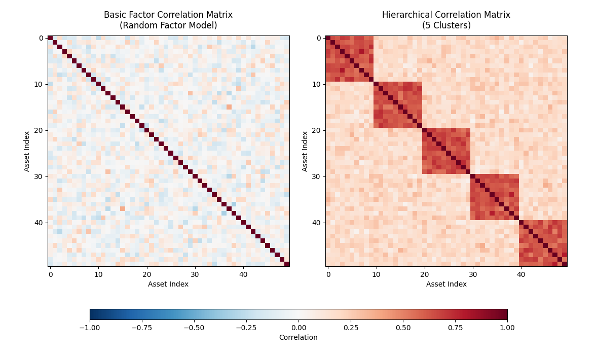
As a sneak preview, we will be generating matrices that look like this:
This approach allows us to assess how cross-sectional systematic strategies behave under different correlation conditions. For instance, in "crisis periods" it is common for correlations of assets to tend towards one. This presents a big risk to portfolios as it significantly hampers diversification. Hence, determining how strategies behave in these periods is very useful for understanding a strategy or portfolio's risk profile.
The first component in our synthetic time series generator to be developed is the class hierarchy for generating correlation matrices. This will subsequently be used to create correlated time series paths under various time series models (some of which we have previously discussed in Brownian Motion Simulation with Python and Geometric Brownian Motion Simulation with Python).
We are going to utilise the concept of an abstract base class (ABC) to produce an interface that all of our derived classes will need to respect. This ensures that we can "swap out" different correlation matrix generator classes, without impacting any of the other modules within the synthetic data generator. This approach has been utilised extensively in our open source QSTrader backtesting software, so if you have previously utilised that tool, you may be familiar with the approach.
We will use this approach for other classes within this tool, including the time series models and correlated path generator components. While it may seem that this introduces undue complexity to our software, we will demonstrate the value of this approach by showing how it can be easily extended to other correlation matrix and time series generation models in subsequent articles.
Abstract Base Class
The first step in defining our class hierarchy is to import the appropriate libraries. We begin the correlation.py file by importing Python's ABC tools, as well as the third party NumPy and SciPy libraries. In particular, we need to import the random_correlation method from the SciPy statistics module:
# correlation.py

from abc import ABC, abstractmethod

import numpy as np
from scipy.stats import random_correlation
We continue the correlation.py file by defining our ABC interface for the CorrelationMatrixGenerator. This has an initialisation method (__init__) that takes in a single argument, $n$, representing the matrix size. We only need to provide a single integer value as the matrix will be $n \times n$. We also add the **kwargs syntax to allow us to add model-specific keyword arguments in more complex matrix generation methods. The method simply creates two class instance attributes n and kwargs:
# ..
# correlation.py
# ..

class CorrelationMatrixGenerator(ABC):
    """
    Abstract base class for correlation matrix generators.
    """

    def __init__(self, n: int, **kwargs):
        """
        Initialize the correlation matrix generator.

        Args:
            n: Size of the correlation matrix (n x n)
            **kwargs: Additional keyword arguments for specific implementations
        """
        self.n = n
        self.kwargs = kwargs
We now providde the first abstract interface method called generate. Decorating this method with @abstractmethod informs Python that any derived subclass must implement this method as there is no default implementation provided. It can be seen that the method is designed to return the generated matrix in the form of a NumPy ndarray, which will contain the actual floating point values of the matrix:
# ..
# correlation.py
# ..

    @abstractmethod
    def generate(self) -> np.ndarray:
        """
        Generate an n x n correlation matrix.
        """
        pass
Continuing with correlation.py, we now provide a method called _make_positive_semidefinite, which is designed to ensure that any randomly generated correlation matrices that we produce respect the mathematical property of positive semidefiniteness. It is worth explaining this aspect briefly, so that the following code is understandable. If you have previously studied linear algebra then you can choose to skip this explanation, otherwise please read on!
Positive semidefiniteness means that when we use the matrix generator classes to generate correlated random data, the results will be meaningful and won't lead to impossible scenarios like negative variances. Without this property, attempting to generate correlated time series could fail or produce nonsensical results.
The method employs eigenvalue decomposition, a linear algebra technique that breaks down the matrix into its fundamental components. This is broadly analogous to decomposing a musical chord into individual notes. Every symmetric matrix (including correlation matrices) can be expressed as a product of three matrices: a matrix of eigenvectors (which represent the "directions" of correlation), a diagonal matrix of eigenvalues (which represent the "strength" along each direction), and the transpose of the eigenvector matrix.
When a correlation matrix isn't positive semidefinite, it has negative eigenvalues, which is problematic. The following algorithm fixes this by setting any negative eigenvalues to a tiny positive value ($10^{-8}$), effectively removing the "impossible" correlations while preserving as much of the original structure as possible. After reconstructing the matrix from these corrected components, it ensures the result remains a valid correlation matrix by normalizing it so all diagonal elements equal exactly 1.0 (since every time series has perfect correlation with itself) and guaranteeing symmetry (since the correlation between A and B must equal the correlation between B and A).
This approach is particularly valuable when correlation matrices are generated through various algorithms or user input, where numerical errors or conflicting specifications might produce mathematically invalid matrices. By applying this correction, the code below ensures that downstream operations, including Cholesky decomposition for generating the actual correlated time series that we will use in subsequent articles, will work reliably without encountering mathematical inconsistencies that could crash the program or produce meaningless output.
The method first obtains the eigenvalues and eigenvectors using NumPy's linalg.eigh method. Then we set all negative values to $10^{-8}$ (a small positive value near zero). Subsequently a new, reconstructed matrix is created by matrix multiplying the eigenvectors with a diagonal matrix of the eigenvalues and the eigenvectors transposed. All values are then normalized to ensure the matrix is a valid correlation matrix. Finally, the diagonals are set equal to unity and the matrix is set to be symmetric:
# ..
# correlation.py
# ..

    def _make_positive_semidefinite(self, matrix: np.ndarray) -> np.ndarray:
        """
        Ensure matrix is positive semidefinite and valid correlation matrix.
        """
        # Eigenvalue decomposition with proper scaling
        eigenvalues, eigenvectors = np.linalg.eigh(matrix)

        # Set negative eigenvalues to small positive value
        eigenvalues[eigenvalues < 0] = 1e-8

        # Reconstruct matrix
        matrix = eigenvectors @ np.diag(eigenvalues) @ eigenvectors.T

        # Normalize to ensure it's a correlation matrix
        # Extract diagonal elements
        d = np.sqrt(np.diag(matrix))

        # Avoid division by zero
        d[d == 0] = 1

        # Normalize
        matrix = matrix / np.outer(d, d)

        # Ensure diagonal is exactly 1 and matrix is symmetric
        np.fill_diagonal(matrix, 1.0)
        matrix = (matrix + matrix.T) / 2

        return matrix
This concludes the implementation of the base CorrelationMatrixGenerator class. On its own this class is not capable of generating any correlation matrices. Instead it is necessary to implement derived subclasses with various models of correlation matrices with varying degrees of realism compared to empirically derived matrices.
Basic Factor Correlation Matrix Generator
The first correlation matrix generator we are going to implement is called the BasicFactorCorrelationGenerator. We will first provide some detail on the underlying rationale for its implementation in the information box below, then will proceed to discuss the code implementation.
The generate method below creates a random correlation matrix using a clever technique based on factor models, which are commonly used in finance to explain how a small number of underlying factors can drive correlations between many assets. If we imagine our time series as being influenced by some hidden common factors plus their own independent variations, the resulting correlation structure will automatically be mathematically valid. This approach sidesteps the difficulty of directly constructing a valid correlation matrix element by element, which often leads to mathematical inconsistencies.
The implementation begins by creating a matrix $W$ of random "factor loadings" with dimensions $n \times k$, where $n$ is the number of variables we want to correlate and $k$ (the random factor parameter) is the number of hidden factors—typically much smaller than $n$. Each row represents how strongly one variable is influenced by each hidden factor. When we multiply this matrix by its transpose (W @ W.T), we get an $n \times n$ matrix that captures how variables become correlated through their shared exposure to common factors. This construction guarantees positive semidefiniteness because any matrix of the form $AA^T$ is automatically positive semidefinite—a fundamental result from linear algebra. The method then adds a tiny diagonal term ($10^{-6}$) for numerical stability, preventing potential issues with near-zero values during subsequent calculations.
The final steps transform this covariance-like matrix into a proper correlation matrix. By dividing each element by the product of the corresponding standard deviations (the square roots of the diagonal elements), we normalize the values to be within the interval $[-1, 1]$, as correlations must. The method ensures the diagonal elements are exactly 1.0 and that the matrix is perfectly symmetric by averaging it with its transpose—addressing any tiny numerical discrepancies from floating-point arithmetic. The np.clip operation provides a final safety net, constraining any values that might have strayed slightly outside the valid $[-1, 1]$ range due to numerical precision limits. This approach generates realistic correlation structures while guaranteeing mathematical validity without needing the correction procedures we saw in the base class.
In the initialisation method __init__ of this class we can see that we are providing an additional integer keyword argument (kwarg) that determines how many random factors affect the correlation matrix:
# ..
# correlation.py
# ..

class BasicFactorCorrelationGenerator(CorrelationMatrixGenerator):
    """
    Basic factor-based correlation matrix generator that creates
    random valid correlation matrices. Uses a method that guarantees
    positive semi-definiteness.
    """

    def __init__(self, n: int, random_factor: int = None, **kwargs):
        """
        Initialize the basic factor correlation generator.

        Args:
            n: Size of the correlation matrix
            random_factor: Factor for random matrix generation
        """
        super().__init__(n, **kwargs)
        self.random_factor = random_factor or max(n + 50, 2 * n)
The following code within the generate method provides the first implementation of the abstract method that was defined within the base class. A matrix $W$ is created initially populated with Guassian (Normal) random values of shape $n \times k$. Then a covariance matrix $S$ is created by matrix multiplying $W$ by its transpose. A small value $10^{-6}$ is added to all diagonals of $S$ by multipling this scalar value by the same-sized identity matrix and adding this to $S$.
The standard deviation of all diagonal values of $S$ are calculated and used to normalize $S$ to obtain a valid correlation matrix. This matrix then has all diagonals set to unity and is ensured to be symmetric. Finally, any values outside of the $[-1, 1]$ interval are clipped to either -1 or 1:
# ..
# correlation.py
# ..

    def generate(self) -> np.ndarray:
        """
        Generate a random valid correlation matrix.
        """
        # Generate random factor loadings and create correlation from them
        # This guarantees a valid correlation matrix

        # Generate random factor loadings matrix
        # More rows than columns ensures positive definiteness
        W = np.random.randn(self.n, self.random_factor)

        # Create covariance matrix
        S = W @ W.T

        # Add small diagonal term for numerical stability
        S += np.eye(self.n) * 1e-6

        # Convert to correlation matrix
        # Extract standard deviations
        std_devs = np.sqrt(np.diag(S))

        # Normalize to get correlation matrix
        corr_matrix = S / np.outer(std_devs, std_devs)

        # Ensure exact properties
        np.fill_diagonal(corr_matrix, 1.0)
        corr_matrix = (corr_matrix + corr_matrix.T) / 2  # Ensure perfect symmetry

        # Clip any numerical errors
        corr_matrix = np.clip(corr_matrix, -1, 1)

        return corr_matrix
This completes the implementation of the BasicFactorCorrelationMatrixGenerator class. While this model is useful for generating basic correlation matrices that can be used to produce synthetic correlated time series, it is far from a realistic model that resembles empirical equities-based correlation matrices.
In order to improve the realism of this model, and demonstrate the ability to "swap out" correlation matrix classes, we are going to develop a further correlation matrix generator model, based on equities sector/industry clustering.
Hierachical Correlation Matrix Generator
The following code snippet implements HierachicalCorrelationMatrixGenerator. The initialisation __init__ method requires a number of kwargs in order to parameterise the model. Specifically, it requires the integer number of sector clusters. It also requires both intra- and inter-cluster correlations, along with a noise value to introduce randomness into these values.
These values can all be modified within configuration (to be defined in a subsequent article) in order to allow you to determine how many sectors you want in your simulated equities asset prices, as well as how correlated their movements are.
# ..
# correlation.py
# ..

class HierarchicalCorrelationMatrixGenerator(CorrelationMatrixGenerator):
    """
    Generates correlation matrices with hierarchical clustering structure.
    This creates blocks of higher correlations to simulate sector/industry clustering.
    """

    def __init__(
        self,
        n: int,
        n_clusters: int = None,
        intra_cluster_corr: float = 0.7,
        inter_cluster_corr: float = 0.2,
        noise_level: float = 0.1,
        **kwargs
    ):
        """
        Initialize the hierarchical correlation generator.

        Args:
            n: Size of the correlation matrix
            n_clusters: Number of clusters (default: sqrt(n))
            intra_cluster_corr: Base correlation within clusters
            inter_cluster_corr: Base correlation between clusters
            noise_level: Amount of random noise to add
        """
        super().__init__(n, **kwargs)
        self.n_clusters = n_clusters or int(np.sqrt(n))
        self.intra_cluster_corr = intra_cluster_corr
        self.inter_cluster_corr = inter_cluster_corr
        self.noise_level = noise_level
As with the BasicFactorCorrelationMatrixGenerator it is necessary to implement the generate function for the HierarchicalCorrelationMatrixGenerator subclass. We will first provide a detailed explanation of the approach we're going to take within the following information box and then we will break down the code.
The HierarchicalCorrelationMatrixGenerator creates correlation matrices that mimic the hierarchical structure commonly observed in financial markets, where assets within the same sector (like technology stocks) tend to move together more strongly than assets from different sectors.
This pattern reflects real-world economic relationships—companies in the same industry face similar market conditions, regulatory changes, and consumer trends, leading to higher correlations within groups than between them. The generator captures this phenomenon by organizing the assets into clusters and assigning different correlation levels based on whether pairs of assets belong to the same cluster or different ones.
The implementation begins by creating a base matrix filled entirely with the inter-cluster correlation value (typically lower, around 0.2), representing the baseline relationship between assets from different sectors. It then divides the $n$ assets into roughly equal clusters, distributing any remainder assets evenly among the clusters.
For each cluster, the algorithm overwrites the corresponding diagonal block of the matrix with the higher intra-cluster correlation value (typically around 0.7), creating visible "blocks" of stronger correlation along the diagonal. This structure directly mimics how a correlation matrix of real market data might look when assets are ordered by sector—bright squares along the diagonal where similar assets cluster together, with dimmer off-diagonal regions representing weaker cross-sector relationships.
To prevent an overly rigid, artificial-looking structure, the method adds random noise drawn from a normal distribution, making the correlation pattern more realistic and varied. The noise is symmetrized by averaging with its transpose to maintain the matrix's required symmetry property (as has been done in the previous basic correlation matrix generator).
After clipping values to ensure they remain within the valid correlation range of $[-1, 1]$ and setting the diagonal to exactly 1.0, the generate method calls the inherited _make_positive_semidefinite function from the base class to guarantee mathematical validity.
The first part of the generate method creates a $n \times n$ matrix full of inter cluster correlation values. The next aspect creates the array of cluster sizes. Subsequently, for each cluster size, the appropriate elements within the matrix are set to the intra cluster correlation value using NumPy slicing notation to ensure the correct sub-block within the matrix is selected. This is achieved by iteratively increasing the start_idx and end_idx values by the size of each cluster.
At this stage the entire matrix values are either set to the inter cluster correlation value or the intra correlation value within certain blocks along the diagonal. In order to make this more realistic, it is necessary to add some variation to these correlation values. To achieve this, some Gaussian noise is added to each value in the matrix for a given standard deviation noise_level. This noise matrix is set to be symmetric and then added to the original correlation matrix.
Finally, all diagonal values are set to unity and the matrix is ensured to be positive semi-definite, as with the previous correlation matrix generator.
# ..
# correlation.py
# ..

    def generate(self) -> np.ndarray:
        """
        Generate a hierarchical correlation matrix.
        """
        # Initialize with inter-cluster correlation
        matrix = np.full((self.n, self.n), self.inter_cluster_corr)

        # Assign assets to clusters
        cluster_sizes = [self.n // self.n_clusters] * self.n_clusters
        # Distribute remaining assets
        for i in range(self.n % self.n_clusters):
            cluster_sizes[i] += 1

        # Create intra-cluster correlations
        start_idx = 0
        for cluster_size in cluster_sizes:
            end_idx = start_idx + cluster_size
            matrix[start_idx:end_idx, start_idx:end_idx] = self.intra_cluster_corr
            start_idx = end_idx

        # Add noise
        noise = np.random.normal(0, self.noise_level, size=(self.n, self.n))
        noise = (noise + noise.T) / 2  # Make symmetric
        matrix += noise

        # Ensure correlations are in [-1, 1]
        matrix = np.clip(matrix, -1, 1)

        # Set diagonal to 1
        np.fill_diagonal(matrix, 1.0)

        # Make positive semidefinite
        matrix = self._make_positive_semidefinite(matrix)

        return matrix
This completes correlation.py. The module has no entrypoint and exists simply to implement that matrix generator classes. In order to actually see what instances of these classes look like in practice, we are going to write a small visualization script that will plot a representative matrix from each of these generators side-by-side in the next section.
Matrix Visualization
To generate visualisations of these two correlation matrix generators we can utilise the Python NumPy and Matplotlib libraries. In particular, we can use the imshow method from Matplotlib to take the two-dimensional NumPy matrix outputs and plot them as a heatmap, with an appropriate colormap.
Since the elements within a correlation matrix are in the interval $[-1, 1]$ it makes more sense to utilise a diverging colormap such as RdBu_r (red-blue reversed), rather than a perceptually uniform map, such as the default viridis. This makes it more straightforward to identify extreme negative and positive correlations by looking for areas of dark red or blue.
We are going to create a separate script called visualization.py which will be placed in the same directory as correlation.py. This short script will demonstrate plotting of samples from each of the correlation matrix generators to provide insight into the types of matrices they can both generate.
The first step is to import the NumPy and Matplotlib libraries, as well as the two generator classes from correlation.py:
# visualization.py

import matplotlib.pyplot as plt
import numpy as np

from correlation import (
    BasicFactorCorrelationMatrixGenerator,
    HierarchicalCorrelationMatrixGenerator
)
We then set a random seed for the NumPy Pseudo Random Number Generator (PRNG), that will ensure that you see exactly the same matrix samples as are shown in the figure below. We set the size of the correlation matrices to be $n=50$, with the hierarchical matrix generator set to use 5 clusters.
We then instantiate both of the correlation matrix generators and call their respective generate methods to obtain a single sample matrix from each class instance:
# ..
# visualization.py
# ..

# Set random seed for reproducibility
np.random.seed(42)

# Parameters
n = 50  # Size of correlation matrices
n_clusters = 5  # Number of clusters for hierarchical generator

# Generate correlation matrices
basic_generator = BasicFactorCorrelationMatrixGenerator(n=n)
basic_matrix = basic_generator.generate()

hierarchical_generator = HierarchicalCorrelationMatrixGenerator(
    n=n,
    n_clusters=n_clusters,
    intra_cluster_corr=0.7,
    inter_cluster_corr=0.2,
    noise_level=0.1
)
hierarchical_matrix = hierarchical_generator.generate()
The remainder of the script is largely used to define all of the various Matplotlib settings for creating a subplot, along with labelling and inclusion of a color bar. We first set up a figure instance, then create two separate axis objects. We then use the Matplotlib imshow method to create two heatmaps (one per axis), with ranges in $[-1, 1]$, using the aforementioned red-blue reversed diverging colormap.
Each of the axes is modified to have a specific sub-title, specific x and y labels and to turn off the default grid. We also adjust the spacing to ensure the plot is sufficiently readable. Finally, we add a color bar to display how the color intensity/hue maps to the correlation values within the matrix.
By default the script will display the plot directly in a separate window (or in a Jupyter Notebook output cell, if running the code within Jupyter). If you would prefer to save the image as a PNG file, then you can uncomment the final line and the correlation matrix plot will be saved to disk:
# ..
# visualization.py
# ..

# Create visualization with adjusted spacing
fig = plt.figure(figsize=(14, 7))

# Create subplot with more space at bottom for colorbar
ax1 = plt.subplot(1, 2, 1)
ax2 = plt.subplot(1, 2, 2)

# Plot basic factor correlation matrix
im1 = ax1.imshow(basic_matrix, cmap='RdBu_r', vmin=-1, vmax=1, aspect='auto')
ax1.set_title('Basic Factor Correlation Matrix\n(Random Factor Model)', fontsize=12, pad=10)
ax1.set_xlabel('Asset Index')
ax1.set_ylabel('Asset Index')
ax1.grid(False)

# Plot hierarchical correlation matrix
im2 = ax2.imshow(hierarchical_matrix, cmap='RdBu_r', vmin=-1, vmax=1, aspect='auto')
ax2.set_title(f'Hierarchical Correlation Matrix\n({n_clusters} Clusters)', fontsize=12, pad=10)
ax2.set_xlabel('Asset Index')
ax2.set_ylabel('Asset Index')
ax2.grid(False)

# Adjust subplot positioning to make room for title and colorbar
plt.subplots_adjust(bottom=0.25, top=0.9, left=0.08, right=0.95, wspace=0.15)

# Add a shared colorbar with better positioning
cbar_ax = fig.add_axes([0.15, 0.1, 0.7, 0.03])  # [left, bottom, width, height]
fig.colorbar(im2, cax=cbar_ax, label='Correlation', orientation='horizontal')

# Display the plot
plt.show()

# Optional: Save the figure
# plt.savefig('correlation_matrices_comparison.png', dpi=150, bbox_inches='tight')
In a suitable virtual environment you can run the following command in the terminal:
$ python3 visualization.pyThe results of this script can be seen in the figure below. The left hand side displays a sample matrix created by the Basic Factor Correlation Matrix Generator, while the right hand side shows a sample matrix created by the Hierarchical Correlation Matrix Generator. It can be seen that the left hand matrix has small randomised off-diagonal entries, while the right hand matrix has a block structure representing the intra sector correlations.
Next Steps
In subsequent articles these generators will be utilised to provide the correlations necessary to generate correlated time series, which will then form the basis of a synthetic data generator for equities data.
These datasets will then be used for the purposes of machine learning model "pre-training", where we will train ML models to generate similar data, prior to "fine-tuning" the models on real financial data.
Full Code
# correlation.py

from abc import ABC, abstractmethod

import numpy as np
from scipy.stats import random_correlation


class CorrelationMatrixGenerator(ABC):
    """
    Abstract base class for correlation matrix generators.
    """

    def __init__(self, n: int, **kwargs):
        """
        Initialize the correlation matrix generator.

        Args:
            n: Size of the correlation matrix (n x n)
            **kwargs: Additional keyword arguments for specific implementations
        """
        self.n = n
        self.kwargs = kwargs

    @abstractmethod
    def generate(self) -> np.ndarray:
        """
        Generate an n x n correlation matrix.
        """
        pass

    def _make_positive_semidefinite(self, matrix: np.ndarray) -> np.ndarray:
        """
        Ensure matrix is positive semidefinite and valid correlation matrix.
        """
        # Eigenvalue decomposition with proper scaling
        eigenvalues, eigenvectors = np.linalg.eigh(matrix)

        # Set negative eigenvalues to small positive value
        eigenvalues[eigenvalues < 0] = 1e-8

        # Reconstruct matrix
        matrix = eigenvectors @ np.diag(eigenvalues) @ eigenvectors.T

        # Normalize to ensure it's a correlation matrix
        # Extract diagonal elements
        d = np.sqrt(np.diag(matrix))

        # Avoid division by zero
        d[d == 0] = 1

        # Normalize
        matrix = matrix / np.outer(d, d)

        # Ensure diagonal is exactly 1 and matrix is symmetric
        np.fill_diagonal(matrix, 1.0)
        matrix = (matrix + matrix.T) / 2

        return matrix


class BasicFactorCorrelationGenerator(CorrelationMatrixGenerator):
    """
    Basic factor-based correlation matrix generator that creates
    random valid correlation matrices. Uses a method that guarantees
    positive semi-definiteness.
    """

    def __init__(self, n: int, random_factor: int = None, **kwargs):
        """
        Initialize the basic factor correlation generator.

        Args:
            n: Size of the correlation matrix
            random_factor: Factor for random matrix generation
        """
        super().__init__(n, **kwargs)
        self.random_factor = random_factor or max(n + 50, 2 * n)

    def generate(self) -> np.ndarray:
        """
        Generate a random valid correlation matrix.
        """
        # Generate random factor loadings and create correlation from them
        # This guarantees a valid correlation matrix

        # Generate random factor loadings matrix
        # More rows than columns ensures positive definiteness
        W = np.random.randn(self.n, self.random_factor)

        # Create covariance matrix
        S = W @ W.T

        # Add small diagonal term for numerical stability
        S += np.eye(self.n) * 1e-6

        # Convert to correlation matrix
        # Extract standard deviations
        std_devs = np.sqrt(np.diag(S))

        # Normalize to get correlation matrix
        corr_matrix = S / np.outer(std_devs, std_devs)

        # Ensure exact properties
        np.fill_diagonal(corr_matrix, 1.0)
        corr_matrix = (corr_matrix + corr_matrix.T) / 2  # Ensure perfect symmetry

        # Clip any numerical errors
        corr_matrix = np.clip(corr_matrix, -1, 1)

        return corr_matrix


class HierarchicalCorrelationMatrixGenerator(CorrelationMatrixGenerator):
    """
    Generates correlation matrices with hierarchical clustering structure.
    This creates blocks of higher correlations to simulate sector/industry clustering.
    """

    def __init__(
        self,
        n: int,
        n_clusters: int = None,
        intra_cluster_corr: float = 0.7,
        inter_cluster_corr: float = 0.2,
        noise_level: float = 0.1,
        **kwargs
    ):
        """
        Initialize the hierarchical correlation generator.

        Args:
            n: Size of the correlation matrix
            n_clusters: Number of clusters (default: sqrt(n))
            intra_cluster_corr: Base correlation within clusters
            inter_cluster_corr: Base correlation between clusters
            noise_level: Amount of random noise to add
        """
        super().__init__(n, **kwargs)
        self.n_clusters = n_clusters or int(np.sqrt(n))
        self.intra_cluster_corr = intra_cluster_corr
        self.inter_cluster_corr = inter_cluster_corr
        self.noise_level = noise_level

    def generate(self) -> np.ndarray:
        """
        Generate a hierarchical correlation matrix.
        """
        # Initialize with inter-cluster correlation
        matrix = np.full((self.n, self.n), self.inter_cluster_corr)

        # Assign assets to clusters
        cluster_sizes = [self.n // self.n_clusters] * self.n_clusters
        # Distribute remaining assets
        for i in range(self.n % self.n_clusters):
            cluster_sizes[i] += 1

        # Create intra-cluster correlations
        start_idx = 0
        for cluster_size in cluster_sizes:
            end_idx = start_idx + cluster_size
            matrix[start_idx:end_idx, start_idx:end_idx] = self.intra_cluster_corr
            start_idx = end_idx

        # Add noise
        noise = np.random.normal(0, self.noise_level, size=(self.n, self.n))
        noise = (noise + noise.T) / 2  # Make symmetric
        matrix += noise

        # Ensure correlations are in [-1, 1]
        matrix = np.clip(matrix, -1, 1)

        # Set diagonal to 1
        np.fill_diagonal(matrix, 1.0)

        # Make positive semidefinite
        matrix = self._make_positive_semidefinite(matrix)

        return matrix
# visualization.py

import matplotlib.pyplot as plt
import numpy as np

from correlation import (
    BasicFactorCorrelationMatrixGenerator,
    HierarchicalCorrelationMatrixGenerator
)


# Set random seed for reproducibility
np.random.seed(42)

# Parameters
n = 50  # Size of correlation matrices
n_clusters = 5  # Number of clusters for hierarchical generator

# Generate correlation matrices
basic_generator = BasicFactorCorrelationMatrixGenerator(n=n)
basic_matrix = basic_generator.generate()

hierarchical_generator = HierarchicalCorrelationMatrixGenerator(
    n=n,
    n_clusters=n_clusters,
    intra_cluster_corr=0.7,
    inter_cluster_corr=0.2,
    noise_level=0.1
)
hierarchical_matrix = hierarchical_generator.generate()


# Create visualization with adjusted spacing
fig = plt.figure(figsize=(14, 7))

# Create subplot with more space at bottom for colorbar
ax1 = plt.subplot(1, 2, 1)
ax2 = plt.subplot(1, 2, 2)

# Plot basic factor correlation matrix
im1 = ax1.imshow(basic_matrix, cmap='RdBu_r', vmin=-1, vmax=1, aspect='auto')
ax1.set_title('Basic Factor Correlation Matrix\n(Random Factor Model)', fontsize=12, pad=10)
ax1.set_xlabel('Asset Index')
ax1.set_ylabel('Asset Index')
ax1.grid(False)

# Plot hierarchical correlation matrix
im2 = ax2.imshow(hierarchical_matrix, cmap='RdBu_r', vmin=-1, vmax=1, aspect='auto')
ax2.set_title(f'Hierarchical Correlation Matrix\n({n_clusters} Clusters)', fontsize=12, pad=10)
ax2.set_xlabel('Asset Index')
ax2.set_ylabel('Asset Index')
ax2.grid(False)

# Adjust subplot positioning to make room for title and colorbar
plt.subplots_adjust(bottom=0.25, top=0.9, left=0.08, right=0.95, wspace=0.15)

# Add a shared colorbar with better positioning
cbar_ax = fig.add_axes([0.15, 0.1, 0.7, 0.03])  # [left, bottom, width, height]
fig.colorbar(im2, cax=cbar_ax, label='Correlation', orientation='horizontal')

# Display the plot
plt.show()

# Optional: Save the figure
# plt.savefig('correlation_matrices_comparison.png', dpi=150, bbox_inches='tight')

