The purpose of this article series is to introduce a very familiar technique, Linear Regression, in a more rigourous mathematical setting under a probabilistic, supervised learning interpretation. This will allow us to understand the probability framework that will subsequently be used for more complex supervised learning models, in a more straightforward setting.
We will initially proceed by defining multiple linear regression, placing it in a probabilistic supervised learning framework and deriving an optimal estimate for its parameters via a technique known as maximum likelihood estimation.
In subsequent articles we will discuss mechanisms to reduce or mitigate the dimensionality of certain datasets via the concepts of subset selection and shrinkage. In addition we will utilise the Python Scitkit-Learn library to demonstrate linear regression, subset selection and shrinkage.
Many of these techniques will naturally carry over to more sophisticated models and will aid us significantly in creating effective, robust statistical methods for trading strategy development.
This article is significantly more mathematically rigourous than other articles have been to date. The rationale for this is to introduce you to the more advanced, probabilistic mechanism which pervades machine learning research. Once you have seen a few examples of simpler models in such a framework, it makes it easier to begin looking at the more advanced ML papers for useful trading ideas.
Linear Regression
Linear regression is one of the most familiar and straightforward statistical techniques. It is often taught at highschool, albeit in a simplified manner. It is also usually the first technique considered when studying supervised learning as it brings up important issues that affect many other supervised models.
Linear regression states that the response value $y$ is a linear function of its feature inputs ${\bf x}$. That is:
\begin{eqnarray} y ({\bf x}) = \beta^T {\bf x} + \epsilon = \sum_{j=0}^p \beta_j x_j + \epsilon \end{eqnarray}
Where $\beta^T, {\bf x} \in \mathbb{R}^{p+1}$ and $\epsilon \sim \mathcal{N}(\mu, \sigma^2)$. That is, $\beta^T$ and ${\bf x}$ are both vectors of dimension $p+1$ and $\epsilon$, the error or residual term, is normally distributed with mean $\mu$ and variance $\sigma^2$. $\epsilon$ represents the difference between the predictions made by the linear regression and the true value of the response variable.
Note that $\beta^T$, which represents the transpose of the vector $\beta$, and ${\bf x}$ are both $p+1$-dimensional, rather than $p$ dimensional, because we need to include an intercept term. $\beta^T = (\beta_0, \beta_1, \ldots, \beta_p)$, while ${\bf x} = (1, x_1, \ldots, x_p)$. We must include the '1' in ${\bf x}$ as a notational "trick".
Probabilistic Interpretation
An alternative way to look at linear regression is to consider it as a joint probability model[2], [3]. That is, we are interested in the joint probability of how the behaviour of the response $y$ is conditional on the values of the feature vector ${\bf x}$, as well as any parameters of the model, given by the vector ${\bf \theta}$. Thus we are interested in a model of the form $p(y \mid {\bf x}, {\bf \theta})$. This is a conditional probability density (CPD) model.
Linear regression can be written as a CPD in the following manner:
\begin{eqnarray} p(y \mid {\bf x}, {\bf \theta}) = \mathcal (y \mid \mu({\bf x}), \sigma^2 ({\bf x})) \end{eqnarray}
For linear regression we assume that $\mu({\bf x})$ is linear and so $\mu ({\bf x}) = \beta^T {\bf x}$. We must also assume that the variance in the model is fixed (i.e. that it doesn't depend on ${\bf x}$) and as such $\sigma^2 ({\bf x}) = \sigma^2$, a constant. This then implies that our parameter vector $\theta = (\beta, \sigma^2)$.
If you recall, we used such a probabilistic interpretation when we considered Bayesian Linear Regression in a previous article.
The benefit of generalising the model interpretation in this manner is that we can easily see how other models, especially those which handle non-linearities, fit into the same probabilistic framework. This allows us to derive results across models using similar techniques.
If we restrict ${\bf x} = (1, x)$, we can make a two-dimensional plot $p(y \mid {\bf x}, {\bf \theta})$ against $y$ and $x$ to see this joint distribution graphically. In order to do so we need to fix the parameters $\beta = (\beta_0, \beta_1)$ and $\sigma^2$ (which constitute the $\theta$ parameters). Here is a Python script which uses matplotlib to display the distribution:
from matplotlib import cm
from matplotlib.ticker import LinearLocator, FormatStrFormatter
import matplotlib.pyplot as plt
import numpy as np
from scipy.stats import norm


if __name__ == "__main__":
    # Set up the X and Y dimensions
    fig = plt.figure()
    ax = fig.gca(projection='3d')
    X = np.arange(0, 20, 0.25)
    Y = np.arange(-10, 10, 0.25)
    X, Y = np.meshgrid(X, Y)

    # Create the univarate normal coefficients
    # of intercep and slope, as well as the
    # conditional probability density
    beta0 = -5.0
    beta1 = 0.5
    Z = norm.pdf(Y, beta0 + beta1*X, 1.0)

    # Plot the surface with the "coolwarm" colormap
    surf = ax.plot_surface(
        X, Y, Z, rstride=1, cstride=1, cmap=cm.coolwarm,
        linewidth=0, antialiased=False
    )

    # Set the limits of the z axis and major line locators
    ax.set_zlim(0, 0.4)
    ax.zaxis.set_major_locator(LinearLocator(5))
    ax.zaxis.set_major_formatter(FormatStrFormatter('%.02f'))

    # Label all of the axes
    ax.set_xlabel('X')
    ax.set_ylabel('Y')
    ax.set_zlabel('P(Y|X)')

    # Adjust the viewing angle and axes direction
    ax.view_init(elev=30., azim=50.0)
    ax.invert_xaxis()
    ax.invert_yaxis()

    # Plot the probability density
    plt.show()
And the output:
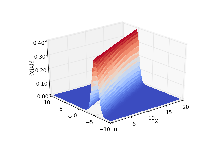 Plot of $p(y \mid {\bf x}, {\bf \theta})$ against $y$ and $x$, influenced from a similar plot in Murphy (2012)[3].
It is clear that the respnse $y$ is linearly dependent upon $x$. However we are also able to ascertain the probabilistic element of the model via the fact that the probability spreads normally around the linear response.
Basis Function Expansion
One of the benefits of utilising the probabilistic interpretation is that it allows us to easily see how to model non-linear relationships, simply by replacing the feature vector ${\bf x}$ with some transformation function $\phi({\bf x})$:
\begin{eqnarray} p(y \mid {\bf x}, {\bf \theta}) = \mathcal(y \mid \beta^T \phi({\bf x}), \sigma^2) \end{eqnarray}
For ${\bf x} = (1, x_1, x_2, x_3)$, say, we could create a $\phi$ that includes higher order terms, including cross-terms, e.g.
\begin{eqnarray} \phi({\bf x}) = (1, x_1, x_1^2, x_2, x^2_2, x_1 x_2, x_3, x_3^2, x_1 x_3, \ldots) \end{eqnarray}
A key point here is that while this function is not linear in the features, ${\bf x}$, it is still linear in the parameters, ${\bf \beta}$ and thus is still called linear regression.
Such a modification, using a transformation function $\phi$, is known as a basis function expansion and can be used to generalise linear regression to many non-linear data settings.
We won't discuss this much further in this article as there are many other more sophisticated supervised learning techniques for capturing non-linearities. We've already discussed one such technique, Support Vector Machines with the "kernel trick", at length in this article.
Maximum Likelihood Estimation
In this section we are going to see how optimal linear regression coefficients, that is the $\beta$ parameter components, are chosen to best fit the data. In the univariate case this is often known as "finding the line of best fit". However, we are in a multivariate case, as our feature vector ${\bf x} \in \mathbb{R}^{p+1}$. Hence we are "finding the $p$-dimensional hyperplane of best fit"!
The main mechanism for finding parameters of statistical models is known as maximum likelihood estimation (MLE). I introduced it briefly in the article on Deep Learning and the Logistic Regression. Here I will expand upon it further.
Likelihood and Negative Log Likelihood
The basic idea is that if the data were to have been generated by the model, what parameters were most likely to have been used? That is, what is the probability of seeing the data $\mathcal{D}$, given a specific set of parameters ${\bf \theta}$? Once again, this is a conditional probability density problem. We are seeking the values of $\theta$ that maximise $p(\mathcal{D} \mid {\bf \theta})$. This CPD is known as the likelihood, and you might recall seeing instances of it in the introductory article on Bayesian statistics.
This problem can be formulated as hunting for the mode of $p(\mathcal{D} \mid {\bf \theta})$, which is given by $\hat{{\bf \theta}}$. For reasons of computational ease we instead try and maximise the natural logarithm of the CPD rather than the CPD itself:
\begin{eqnarray} \hat{{\bf \theta}} = \text{argmax}_{\theta} \log p(\mathcal{D} \mid {\bf \theta}) \end{eqnarray}
In linear regression problems we need to make the assumption that the feature vectors are all independent and identically distributed (iid). This makes it far simpler to solve the log-likelihood problem, using properties of natural logarithms. Since we will be differentiating these values it is far easier to differentiate a sum than a product, hence the logarithm:
\begin{eqnarray} \mathcal{l}({\bf \theta}) &:=& \log p(\mathcal{D} \mid {\bf \theta}) \\ &=& \log \left( \prod_{i=1}^{N} p(y_i \mid {\bf x}_i, {\bf \theta}) \right) \\ &=& \sum_{i=1}^{N} \log p(y_i \mid {\bf x}_i, {\bf \theta}) \end{eqnarray}
As I also mentioned in the article on Deep Learning/Logistic Regression, for reasons of increased computational ease, it is often easier to minimise the negative of the log-likelihood rather than maximise the log-likelihood itself. Hence, we can "stick a minus sign in front of the log-likelihood" to give us the negative log-likelihood (NLL):
\begin{eqnarray} \text{NLL} ({\bf \theta}) = - \sum_{i=1}^{N} \log p(y_i \mid {\bf x}_i, {\bf \theta}) \end{eqnarray}
This is the function we need to minimise. By doing so we will derive the ordinary least squares estimate for the $\beta$ coefficients.
Ordinary Least Squares
Our goal here is to derive the optimal set of $\beta$ coefficients that are "most likely" to have generated the data for our training problem. These coefficients will allow us to form a hyperplane of "best fit" through the training data. The process we will follow is given by:
- Use the definition of the normal distribution to expand the negative log likelihood function
- Utilise the properties of logarithms to reformulate this in terms of the Residual Sum of Squares (RSS), which is equivalent to the sum of each residual across all observations
- Rewrite the residuals in matrix form, creating the data matrix $X$, which is $N \times (p+1)$ dimensional, and formulate the RSS as a matrix equation
- Differentiate this matrix equation with respect to (w.r.t) the parameter vector $\beta$ and set the equation to zero (with some assumptions on $X$)
- Solve the subsequent equation for $\beta$ to receive $\hat{\beta}_\text{OLS}$, the ordinary least squares (OLS) estimate.
The next section will closely follow the treatments of [2] and [3]. The first step is to expand the NLL using the formula for a normal distribution:
\begin{eqnarray} \text{NLL} ({\bf \theta}) &=& - \sum_{i=1}^{N} \log p(y_i \mid {\bf x}_i, {\bf \theta}) \\ &=& - \sum_{i=1}^{N} \log \left[ \left(\frac{1}{2 \pi \sigma^2}\right)^{\frac{1}{2}} \exp \left( - \frac{1}{2 \sigma^2} (y_i - {\bf \beta}^{T} {\bf x}_i)^2 \right)\right] \\ &=& - \sum_{i=1}^{N} \frac{1}{2} \log \left( \frac{1}{2 \pi \sigma^2} \right) - \frac{1}{2 \sigma^2} (y_i - {\bf \beta}^T {\bf x}_i)^2 \\ &=& - \frac{N}{2} \log \left( \frac{1}{2 \pi \sigma^2} \right) - \frac{1}{2 \sigma^2} \sum_{i=1}^N (y_i - {\bf \beta}^T {\bf x}_i)^2 \\ &=& - \frac{N}{2} \log \left( \frac{1}{2 \pi \sigma^2} \right) - \frac{1}{2 \sigma^2} \text{RSS}({\bf \beta}) \end{eqnarray}
Where $\text{RSS}({\bf \beta}) := \sum_{i=1}^N (y_i - {\bf \beta}^T {\bf x}_i)^2$ is the Residual Sum of Squares, also known as the Sum of Squared Errors (SSE).
Since the first term in the equation is a constant we simply need to concern ourselves with minimising the RSS, which will be sufficient for producing the optimal parameter estimate.
To simply the notation we can write this latter term in matrix form. By defining the $N \times (p+1)$ matrix $X$ we can write the RSS term as:
\begin{eqnarray} \text{RSS}({\bf \beta}) = ({\bf y} - {\bf X}{\bf \beta})^T ({\bf y} - {\bf X}{\bf \beta}) \end{eqnarray}
At this stage we now want to differentiate this term w.r.t. the parameter variable ${\bf \beta}$:
\begin{eqnarray} \frac{\partial RSS}{\partial \beta} = -2 {\bf X}^T ({\bf y} - {\bf X} \beta) \end{eqnarray}
There is an extremely key assumption to make here. We need ${\bf X}^T {\bf X}$ to be positive-definite, which is only the case if there are more observations than there are dimensions. If this is not the case (which is extremely common in high-dimensional settings) then it is not possible to find a unique set of $\beta$ coefficients and thus the following matrix equation will not hold.
Under the assumption of a positive-definite ${\bf X}^T {\bf X}$ we can set the differentiated equation to zero and solve for $\beta$:
\begin{eqnarray} {\bf X}^T ({\bf y} - {\bf X} \beta) = 0 \end{eqnarray}
The solution to this matrix equation provides $\hat{\beta}_\text{OLS}$:
\begin{eqnarray} \hat{\beta}_\text{OLS} = ({\bf X}^{T} {\bf X})^{-1} {\bf X}^{T} {\bf y} \end{eqnarray}
Next Steps
Now that we have considered the MLE procedure for producing the OLS estimates we are in a position to discuss what happens when we are in a high-dimensional setting (as is often the case with real world data) and thus our matrix ${\bf X}^T {\bf X}$ has no inverse. In this instance we need to use subset selection and shrinkage techniques to reduce the dimensionality of the problem. This will be the subject of the next article.
Bibliographic Note
An elementary introduction to linear regression, as well as shrinkage, regularisation and dimensionality redution, in the framework of supervised learning, can be found [1]. For a much more rigourous explanation of the techniques, including recent developments, can be found in [2]. A probabilistic (mainly Bayesian) approach to linear regression, along with a comprehensive derivation of the maximum likelihood estimate via ordinary least squares, and extensive discussion of shrinkage and regularisation, can be found in [3]. A "real world" example-based overview of linear regression in a high-collinearity regime, with extensive discussion on dimensionality reduction and partial least squares can be found in [4].
References
- [1] James, G., Witten, D., Hastie, T., Tibshirani, R. (2013) An Introduction to Statistical Learning, Springer
- [2] Hastie, T., Tibshirani, R., Friedman, J. (2009) The Elements of Statistical Learning, Springer
- [3] Murphy, K.P. (2012) Machine Learning A Probabilistic Perspective, MIT Press
- [4] Kuhn, M., Johnson, K. (2013) Applied Predictive Modelling, Springer


