In the previous article on the Cointegrated Augmented Dickey Fuller (CADF) test we noted that one of the biggest drawbacks of the test was that it was only capable of being applied to two separate time series. However, we can clearly imagine a set of three or more financial assets that might share an underlying cointegrated relationship.
A trivial example would be three separate share classes on the same asset, while a more interesting example would be three separate ETFs that all track certain areas of commodity equities and the underlying commodity spot prices.
In this article we are going to discuss a test due to Johansen[3] that allows us to determine if three or more time series are cointegrated. We will then form a stationary series by taking a linear combination of the underlying series. Such a procedure will be utilised in subsequent articles to form a mean reverting portfolio of assets for trading purposes.
We will begin by describing the theory underlying the Johansen test and then perform our usual procedure of carrying out the test on simulated data with known cointegrating properties. Subsequently we will apply the test to historical financial data and see if we can find a portfolio of cointegrated assets.
Johansen Test
In this section we will outline the mathematical underpinnings of the Johansen procedure, which allows us to analyse whether two or more time series can form a cointegrating relationship. In quantitative trading this would allow us to form a portfolio of two or more securities in a mean reversion trading strategy.
The theoretical details of the Johansen test require a bit of experience with multivariate time series, which we have not considered to date on QuantStart. In particular we need to consider Vector Autoregressive Models (VAR) - not to be confused with Value at Risk (VaR) - which are a multidimensional extension of the Autoregressive Models studied previously.
A general vector autoregressive model is similar to the AR(p) model except that each quantity is vector valued and matrices are used as the coefficients. The general form of the VAR(p) model, without drift, is given by:
\begin{eqnarray} {\bf x_t} = {\bf \mu} + A_1 {\bf x_{t-1}} + \ldots + A_p {\bf x_{t-p}} + {\bf w_t} \end{eqnarray}
Where ${\bf \mu}$ is the vector-valued mean of the series, $A_i$ are the coefficient matrices for each lag and ${\bf w_t}$ is a multivariate Gaussian noise term with mean zero.
At this stage we can form a Vector Error Correction Model (VECM) by differencing the series:
\begin{eqnarray} \Delta {\bf x_t} = {\bf \mu} + A {\bf x_{t-1}} + \Gamma_1 \Delta {\bf x_{t-1}} + \ldots + \Gamma_p \Delta {\bf x_{t-p}} + {\bf w_t} \end{eqnarray}
Where $\Delta {\bf x_t} := {\bf x_t} - {\bf x_{t-1}}$ is the differencing operator, $A$ is the coefficient matrix for the first lag and $\Gamma_i$ are the matrices for each differenced lag.
The test checks for the situation of no cointegration, which occurs when the matrix $A=0$.
The Johansen test is more flexible than the CADF procedure outlined in the previous article and can check for multiple linear combinations of time series for forming stationary portfolios.
To achieve this an eigenvalue decomposition of $A$ is carried out. The rank of the matrix $A$ is given by $r$ and the Johansen test sequentially tests whether this rank $r$ is equal to zero, equal to one, through to $r=n-1$, where $n$ is the number of time series under test.
The null hypothesis of $r=0$ means that there is no cointegration at all. A rank $r \gt 0$ implies a cointegrating relationship between two or possibly more time series.
The eigenvalue decomposition results in a set of eigenvectors. The components of the largest eigenvector admits the important property of forming the coefficients of a linear combination of time series to produce a stationary portfolio. Notice how this differs from the CADF test (often known as the Engle-Granger procedure) where it is necessary to ascertain the linear combination a priori via linear regression and ordinary least squares (OLS).
In the Johansen test the linear combination values are estimated as part of the test, which implies that there is less statistical power associated with the test when compared to CADF. It is possible to run into situations where there is insufficient evidence to reject the null hypothesis of no cointegration despite the CADF suggesting otherwise. This will be discussed further below.
Perhaps the best way to understand the Johansen test is to see it applied to both simulated, and historical, financial data.
Johansen Test on Simulated Data
Now that we've outlined the theory of the test we are going to apply it using the R statistical environment. We will make use of the urca library, written by Bernhard Pfaff and Matthieu Stigler, which wraps up the Johansen test in an easy to call function - ca.jo.
The first task is to import the urca library itself:
library("urca")
As in the previous cointegration articles we set the seed so that the results of the random number generator can be replicated in other R environments:
set.seed(123)
We then create the underlying random walk $z_t$ as in previous articles:
z <- rep(0, 10000)
for (i in 2:10000) z[i] <- z[i-1] + rnorm(1)
We create three time series that share the underlying random walk structure from $z_t$. They are denoted by $p_t$, $q_t$ and $r_t$, respectively:
p <- q <- r <- rep(0, 10000)
p <- 0.3*z + rnorm(10000)
q <- 0.6*z + rnorm(10000)
r <- 0.2*z + rnorm(10000)
We then call the ca.jo function applied to a data frame of all three time series.
The type parameter tells the function whether to use the trace test statistic or the maximum eigenvalue test statistic, which are the two separate forms of the Johansen test. In this instance we're using trace.
K is the number of lags to use in the vector autoregressive model and is set this to the minimum, K=2.
ecdet refers to whether to use a constant or drift term in the model, while spec="longrun" refers to the specification of the VECM discussed above. This parameter can be spec="longrun" or spec="transitory".
Finally, we print the summary of the output:
jotest=ca.jo(data.frame(p,q,r), type="trace", K=2, ecdet="none", spec="longrun")
summary(jotest)
The output is as follows:
######################
# Johansen-Procedure #
######################

Test type: trace statistic , with linear trend

Eigenvalues (lambda):
[1] 0.338903321 0.330365610 0.001431603

Values of teststatistic and critical values of test:

            test 10pct  5pct  1pct
r <= 2 |   14.32  6.50  8.18 11.65
r <= 1 | 4023.76 15.66 17.95 23.52
r = 0  | 8161.48 28.71 31.52 37.22

Eigenvectors, normalised to first column:
(These are the cointegration relations)

          p.l2        q.l2     r.l2
p.l2  1.000000  1.00000000 1.000000
q.l2  1.791324 -0.52269002 1.941449
r.l2 -1.717271  0.01589134 2.750312

Weights W:
(This is the loading matrix)

          p.l2         q.l2          r.l2
p.d -0.1381095 -0.771055116 -0.0003442470
q.d -0.2615348  0.404161806 -0.0006863351
r.d  0.2439540 -0.006556227 -0.0009068179
Let's try and interpret all of this information! The first section shows the eigenvalues generated by the test. In this instance we have three with the largest approximately equal to 0.3389.
The next section shows the trace test statistic for the three hypotheses of $r \leq 2$, $r \leq 1$ and $r = 0$. For each of these three tests we have not only the statistic itself (given under the test column) but also the critical values at certain levels of confidence: 10%, 5% and 1% respectively.
The first hypothesis, $r = 0$, tests for the presence of cointegration. It is clear that since the test statistic exceeds the 1% level significantly ($8161.48 \gt 37.22$) that we have strong evidence to reject the null hypothesis of no cointegration. The second test for $r \leq 1$ against the alternative hypothesis of $r \gt 1$ also provides clear evidence to reject $r \leq 1$ since the test statistic exceeds the 1% level significantly. The final test for $r \leq 2$ against $r \gt 2$ also provides sufficient evidence for rejecting the null hypothesis that $r \leq 2$ and so can conclude that the rank of the matrix $r$ is greater than 2.
Thus the best estimate of the rank of the matrix is $r=3$, which tells us that we need a linear combination of three time series to form a stationary series. This is to be expected, by definition of the series, as the underlying random walk utilised for all three series is non-stationary.
How do we go about forming such a linear combination? The answer is to make use of the eigenvector components of the eigenvector associated with the largest eigenvalue. We previously mentioned that the largest eigenvalue is approximately 0.3389. It corresponds to the vector given under the column p.l2, and is approximately equal to $(1.000000, 1.791324, -1.717271)$. If we form a linear combination of series using these components, we will receive a stationary series:
s = 1.000*p + 1.791324*q - 1.717271*r
plot(s, type="l")
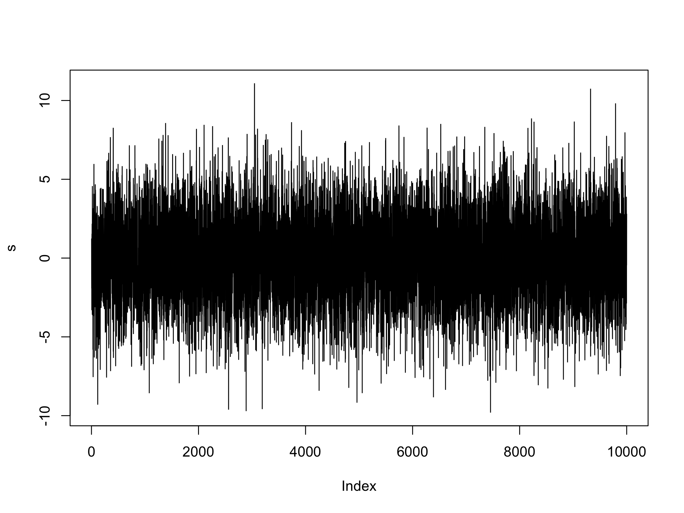 Plot of $s_t$, the stationary series formed via a linear combination of $p_t$, $q_t$ and $r_t$
Visually this looks very much like a stationary series. We can import the Augmented Dickey-Fuller (ADF) test as an additional check:
library("tseries")
adf.test(s)
The output is as follows:
    Augmented Dickey-Fuller Test

data:  s
Dickey-Fuller = -22.0445, Lag order = 21, p-value = 0.01
alternative hypothesis: stationary

Warning message:
In adf.test(s) : p-value smaller than printed p-value
The Dickey-Fuller test statistic is very low, providing a low p-value and hence evidence to reject the null hypothesis of a unit root and thus evidence we have a stationary series formed from a linear combination.
This should not surprise us at all as, by construction, the set of series was designed to form such a linear stationary combination. However, it is instructive to follow the tests through on simulated data as it helps us when analysing real financial data, as we will be doing so in the next section.
Johansen Test on Financial Data
In this section we will look at two separate sets of ETF baskets: EWA, EWC and IGE as well as SPY, IVV and VOO.
EWA, EWC and IGE
In the previous article we looked at Ernest Chan's[1] work on the cointegration between the two ETFS of EWA and EWC, representing baskets of equities for the Australian and Canadian economies, respectively.
He also discusses the Johansen test as a means of adding a third ETF into the mix, namely IGE, which contains a basket of natural resource stocks. The logic is that all three should in some part be affected by stochastic trends in commodities and thus may form a cointegrating relationship.
In Ernie's work he carried out the Johansen procedure using MatLab and was able to reject the hypothesis of $r \leq 2$ at the 5% level. Recall that this implies that he found evidence to support the existence of a stationary linear combination of EWA, EWC and IGE.
It would be useful to see if we can replicate the results using ca.jo in R. In order to do so we need to use the quantmod library:
library("quantmod")
We now need to obtain backward-adjusted daily closing prices for EWA, EWC and IGE for the same time period that Ernie used:
getSymbols("EWA", from="2006-04-26", to="2012-04-09")
getSymbols("EWC", from="2006-04-26", to="2012-04-09")
getSymbols("IGE", from="2006-04-26", to="2012-04-09")
We also need to create new variables to hold the backward-adjusted prices:
ewaAdj = unclass(EWA$EWA.Adjusted)
ewcAdj = unclass(EWC$EWC.Adjusted)
igeAdj = unclass(IGE$IGE.Adjusted)
We can now perform the Johansen test on the three ETF daily price series and output the summary of the test:
jotest=ca.jo(data.frame(ewaAdj,ewcAdj,igeAdj), type="trace", K=2, ecdet="none", spec="longrun")
summary(jotest)
The output is as follows:
######################
# Johansen-Procedure #
######################

Test type: trace statistic , with linear trend

Eigenvalues (lambda):
[1] 0.011751436 0.008291262 0.002929484

Values of teststatistic and critical values of test:

          test 10pct  5pct  1pct
r <= 2 |  4.39  6.50  8.18 11.65
r <= 1 | 16.87 15.66 17.95 23.52
r = 0  | 34.57 28.71 31.52 37.22

Eigenvectors, normalised to first column:
(These are the cointegration relations)

                EWA.Adjusted.l2 EWC.Adjusted.l2 IGE.Adjusted.l2
EWA.Adjusted.l2       1.0000000        1.000000        1.000000
EWC.Adjusted.l2      -1.1245355        3.062052        3.925659
IGE.Adjusted.l2       0.2472966       -2.958254       -1.408897

Weights W:
(This is the loading matrix)

               EWA.Adjusted.l2 EWC.Adjusted.l2 IGE.Adjusted.l2
EWA.Adjusted.d    -0.007134366     0.004087072   -0.0011290139
EWC.Adjusted.d     0.020630544     0.004262285   -0.0011907498
IGE.Adjusted.d     0.026326231     0.010189541   -0.0009097034
Perhaps the first thing to notice is that the values of the trace test statistic differ from those given in the MatLab jplv7 package used by Ernie. This is most likely because the ca.jo R function in the urca package requires our lag order to be two or greater (K=2), whereas in the MatLab equivalent it is possible to use a lag of unity (K=1).
Our trace test statistic is broadly similar for $r \leq 2$ at 4.39 versus 4.471 for Ernie's results. However the critical values are quite different, with ca.jo having a value of 8.18 at the 95% level for the $r \leq 2$ hypothesis, while the jplv7 package gives 3.841. Crucially Ernie's test statistic is greater than at the 5% level, while ours is lower. Hence we do not have sufficient evidence to reject the null hypothesis of $r \leq 2$ for $K=2$ lags.
The key issue here is that there is no difference between the two sets of time series used for each analysis! The only difference is that the implementations of the Johansen test are different between R's urca and MatLab's jplv7. This means we need to be extremely careful when evaluating the results of statistical tests, especially between differing implementations and programming languages.
If you want to read more about some of the issues when using the Johansen test as compared to the Cointegrated Augmented Dickey-Fuller test, it is worth reading this thread, which has Bernhard Pfaff (co-author of urca) and Eric Zivot (Professor of Economics at University of Washington) weigh in on the test.
SPY, IVV and VOO
Another approach is to consider a basket of ETFs that track an equity index. For instance, there are a multitude of ETFs that track the US S&P500 stock market index such as Standard & Poor's Depository Receipts SPY, the iShares IVV and Vanguard's VOO. Given that they all track the same underlying asset it is likely that these three ETFs will have a strong cointegrating relationship.
Let's obtain the daily adjusted closing prices for each of these ETFs over the last year:
getSymbols("SPY", from="2015-01-01", to="2015-12-31")
getSymbols("IVV", from="2015-01-01", to="2015-12-31")
getSymbols("VOO", from="2015-01-01", to="2015-12-31")
As with EWC, EWA and IGE, we need to utilise the backward adjusted prices:
spyAdj = unclass(SPY$SPY.Adjusted)
ivvAdj = unclass(IVV$IVV.Adjusted)
vooAdj = unclass(VOO$VOO.Adjusted)
Finally, let's run the Johansen test with the three ETFs and output the results:
jotest=ca.jo(data.frame(spyAdj,ivvAdj,vooAdj), type="trace", K=2, ecdet="none", spec="longrun")
summary(jotest)
The output is as follows:
######################
# Johansen-Procedure #
######################

Test type: trace statistic , with linear trend

Eigenvalues (lambda):
[1] 0.29311420 0.24149750 0.04308716

Values of teststatistic and critical values of test:

           test 10pct  5pct  1pct
r <= 2 |  11.01  6.50  8.18 11.65
r <= 1 |  80.11 15.66 17.95 23.52
r = 0  | 166.83 28.71 31.52 37.22

Eigenvectors, normalised to first column:
(These are the cointegration relations)

                SPY.Adjusted.l2 IVV.Adjusted.l2 VOO.Adjusted.l2
SPY.Adjusted.l2       1.0000000        1.000000       1.0000000
IVV.Adjusted.l2      -0.3669563       -4.649203      -0.5170538
VOO.Adjusted.l2      -0.6783666        4.042139      -0.2426406

Weights W:
(This is the loading matrix)

               SPY.Adjusted.l2 IVV.Adjusted.l2 VOO.Adjusted.l2
SPY.Adjusted.d      -1.8692017       0.2875776      -0.3086708
IVV.Adjusted.d      -1.2062706       0.3965064      -0.3160481
VOO.Adjusted.d      -0.9414142       0.2182340      -0.2871731
As before we sequentially carry out the hypothesis tests beginning with the null hypoothesis of $r = 0$ versus the alternative hypothesis of $r \gt 0$. There is clear evidence to reject the null hypothesis at the 1% level and we can likely conclude that $r \gt 0$.
Similarly when we carry out the $r \leq 1$ null hypothesis versus the $r \gt 1$ alternative hypothesis we have sufficient evidence to reject the null hypothesis at the 1% level and can conclude $r \gt 1$.
However, for the $r \leq 2$ hypothesis we can only reject the null hypothesis at the 5% level. This is weaker evidence than the previous hypotheses and, although it suggests we can reject the null at this level, we should be careful that $r$ might equal two, rather than exceed two. What this means is that it may be possible to form a linear combination with only two assets rather than requiring all three to form a cointegrating portfolio.
In addition we should be extremely cautious of interpreting these results as I have only used one years worth of data, which is approximately 250 trading days. Such a small sample is unlikely to provide a true representation of the underlying relationships. Hence, we must always be careful in interpreting statistical tests!
Next Steps
Over the last few articles we've covered a multitude of statistical tests for detecting stationarity among combinations of time series as a precursor to forming mean reversion trading strategies.
In particular we've looked at the Augmented Dickey-Fuller, Phillips-Perron, Phillips-Ouliaris, Cointegrated Augmented Dickey-Fuller and the Johansen test.
We are now in a position to apply these tests to mean reverting strategies. To do so we will form both a for-loop backtest using R and a realistic backtest using QSTrader in Python for these strategies. We will carry out these backtests in subsequent articles.
References
- [1] Chan, E. P. (2013) Algorithmic Trading: Winning Strategies and their Rationale, Wiley
- [2] Turan, D. (2013) Cointegration Tests (ADF and Johansen) within R
- [3] Johansen, S. (1991) Estimation and Hypothesis Testing of Cointegration Vectors in Gaussian Vector Autoregressive Models, Econometrica 59 (6): 1551-1580
Full Code
library("quantmod")
library("tseries")
library("urca")

set.seed(123)

## Simulated cointegrated series

z <- rep(0, 10000)
for (i in 2:10000) z[i] <- z[i-1] + rnorm(1)

p <- q <- r <- rep(0, 10000)

p <- 0.3*z + rnorm(10000)
q <- 0.6*z + rnorm(10000)
r <- 0.8*z + rnorm(10000)

jotest=ca.jo(data.frame(p,q,r), type="trace", K=2, ecdet="none", spec="longrun")
summary(jotest)

s = 1.000*p + 1.791324*q - 1.717271*r
plot(s, type="l")

adf.test(s)

## EWA, EWC and IGE

getSymbols("EWA", from="2006-04-26", to="2012-04-09")
getSymbols("EWC", from="2006-04-26", to="2012-04-09")
getSymbols("IGE", from="2006-04-26", to="2012-04-09")

ewaAdj = unclass(EWA$EWA.Adjusted)
ewcAdj = unclass(EWC$EWC.Adjusted)
igeAdj = unclass(IGE$IGE.Adjusted)

jotest=ca.jo(data.frame(ewaAdj,ewcAdj,igeAdj), type="trace", K=2, ecdet="none", spec="longrun")
summary(jotest)

## SPY, IVV and VOO

getSymbols("SPY", from="2015-01-01", to="2015-12-31")
getSymbols("IVV", from="2015-01-01", to="2015-12-31")
getSymbols("VOO", from="2015-01-01", to="2015-12-31")

spyAdj = unclass(SPY$SPY.Adjusted)
ivvAdj = unclass(IVV$IVV.Adjusted)
vooAdj = unclass(VOO$VOO.Adjusted)

jotest=ca.jo(data.frame(spyAdj,ivvAdj,vooAdj), type="trace", K=2, ecdet="none", spec="longrun")
summary(jotest)


