In the last article we looked at random walks and white noise as basic time series models for certain financial instruments, such as daily equity and equity index prices. We found that in some cases a random walk model was insufficient to capture the full autocorrelation behaviour of the instrument, which motivates more sophisticated models.
In the next couple of articles we are going to discuss three types of model, namely the Autoregressive (AR) model of order $p$, the Moving Average (MA) model of order $q$ and the mixed Autogressive Moving Average (ARMA) model of order $p, q$. These models will help us attempt to capture or "explain" more of the serial correlation present within an instrument. Ultimately they will provide us with a means of forecasting the future prices.
However, it is well known that financial time series possess a property known as volatility clustering. That is, the volatility of the instrument is not constant in time. The technical term for this behaviour is known as conditional heteroskedasticity. Since the AR, MA and ARMA models are not conditionally heteroskedastic, that is, they don't take into account volatility clustering, we will ultimately need a more sophisticated model for our predictions.
Such models include the Autogressive Conditional Heteroskedastic (ARCH) model and Generalised Autogressive Conditional Heteroskedastic (GARCH) model, and the many variants thereof. GARCH is particularly well known in quant finance and is primarily used for financial time series simulations as a means of estimating risk.
However, as with all QuantStart articles, I want to build up to these models from simpler versions so that we can see how each new variant changes our predictive ability. Despite the fact that AR, MA and ARMA are relatively simple time series models, they are the basis of more complicated models such as the Autoregressive Integrated Moving Average (ARIMA) and the GARCH family. Hence it is important that we study them.
One of our first trading strategies in the time series article series will be to combine ARIMA and GARCH in order to predict prices $n$ periods in advance. However, we will have to wait until we've discussed both ARIMA and GARCH separately before we apply them to a real strategy!
How Will We Proceed?
In this article we are going to outline some new time series concepts that we'll need for the remaining methods, namely strict stationarity and the Akaike information criterion (AIC).
Subsequent to these new concepts we will follow the traditional pattern for studying new time series models:
- Rationale - The first task is to provide a reason why we're interested in a particular model, as quants. Why are we introducing the time series model? What effects can it capture? What do we gain (or lose) by adding in extra complexity?
- Definition - We need to provide the full mathematical definition (and associated notation) of the time series model in order to minimise any ambiguity.
- Second Order Properties - We will discuss (and in some cases derive) the second order properties of the time series model, which includes its mean, its variance and its autocorrelation function.
- Correlogram - We will use the second order properties to plot a correlogram of a realisation of the time series model in order to visualise its behaviour.
- Simulation - We will simulate realisations of the time series model and then fit the model to these simulations to ensure we have accurate implementations and understand the fitting process.
- Real Financial Data - We will fit the time series model to real financial data and consider the correlogram of the residuals in order to see how the model accounts for serial correlation in the original series.
- Prediction - We will create $n$-step ahead forecasts of the time series model for particular realisations in order to ultimately produce trading signals.
Nearly all of the articles I write on time series models will fall into this pattern and it will allow us to easily compare the differences between each model as we add further complexity.
We're going to start by looking at strict stationarity and the AIC.
Strictly Stationary
We provided the definition of stationarity in the article on serial correlation. However, because we are going to be entering the realm of many financial series, with various frequencies, we need to make sure that our (eventual) models take into account the time-varying volatility of these series. In particular, we need to consider their heteroskedasticity.
We will come across this issue when we try to fit certain models to historical series. Generally, not all of the serial correlation in the residuals of fitted models can be accounted for without taking heteroskedasticity into account. This brings us back to stationarity. A series is not stationary in the variance if it has time-varying volatility, by definition.
This motivates a more rigourous definition of stationarity, namely strict stationarity:
Strictly Stationary Series
A time series model, $\{ x_t \}$, is strictly stationary if the joint statistical distribution of the elements $x_{t_1},\ldots,x_{t_n}$ is the same as that of $x_{t_{1}+m},\ldots,x_{t_{n}+m}$, $\forall t_i, m$.
One can think of this definition as simply that the distribution of the time series is unchanged for any abritrary shift in time.
In particular, the mean and the variance are constant in time for a strictly stationary series and the autocovariance between $x_t$ and $x_s$ (say) depends only on the absolute difference of $t$ and $s$, $|t-s|$.
We will be revisiting strictly stationary series in future posts.
Akaike Information Criterion
I mentioned in previous articles that we would eventually need to consider how to choose between separate "best" models. This is true not only of time series analysis, but also of machine learning and, more broadly, statistics in general.
The two main methods we will use (for the time being) are the Akaike Information Criterion (AIC) and the Bayesian Information Criterion (as we progress further with our articles on Bayesian Statistics).
We'll briefly consider the AIC, as it will be used in Part 2 of the ARMA article.
AIC is essentially a tool to aid in model selection. That is, if we have a selection of statistical models (including time series), then the AIC estimates the "quality" of each model, relative to the others that we have available.
It is based on information theory, which is a highly interesting, deep topic that unfortunately we can't go into too much detail about. It attempts to balance the complexity of the model, which in this case means the number of parameters, with how well it fits the data. Let's provide a definition:
Akaike Information Criterion
If we take the likelihood function for a statistical model, which has $k$ parameters, and $L$ maximises the likelihood, then the Akaike Information Criterion is given by:
\begin{eqnarray} AIC = -2 \text{log} (L) + 2k \end{eqnarray}The preferred model, from a selection of models, has the minium AIC of the group. You can see that the AIC grows as the number of parameters, $k$, increases, but is reduced if the negative log-likelihood increases. Essentially it penalises models that are overfit.
We are going to be creating AR, MA and ARMA models of varying orders and one way to choose the "best" model fit a particular dataset is to use the AIC. This is what we'll be doing in the next article, primarily for ARMA models.
Autoregressive (AR) Models of order p
The first model we're going to consider, which forms the basis of Part 1, is the Autoregressive model of order $p$, often shortened to AR(p).
Rationale
In the previous article we considered the random walk, where each term, $x_t$ is dependent solely upon the previous term, $x_{t-1}$ and a stochastic white noise term, $w_t$:
\begin{eqnarray} x_t = x_{t-1} + w_t \end{eqnarray}The autoregressive model is simply an extension of the random walk that includes terms further back in time. The structure of the model is linear, that is the model depends linearly on the previous terms, with coefficients for each term. This is where the "regressive" comes from in "autoregressive". It is essentially a regression model where the previous terms are the predictors.
Autoregressive Model of order p
A time series model, $\{ x_t \}$, is an autoregressive model of order $p$, AR(p), if:
\begin{eqnarray} x_t &=& \alpha_1 x_{t-1} + \ldots + \alpha_p x_{t-p} + w_t \\ &=& \sum_{i=1}^p \alpha_i x_{t-i} + w_t \end{eqnarray}Where $\{ w_t \}$ is white noise and $\alpha_i \in \mathbb{R}$, with $\alpha_p \neq 0$ for a $p$-order autoregressive process.
If we consider the Backward Shift Operator, ${\bf B}$ (see previous article) then we can rewrite the above as a function $\theta$ of ${\bf B}$:
\begin{eqnarray} \theta_p ({\bf B}) x_t = (1 - \alpha_1 {\bf B} - \alpha_2 {\bf B}^2 - \ldots - \alpha_p {\bf B}) x_t = w_t \end{eqnarray}Perhaps the first thing to notice about the AR(p) model is that a random walk is simply AR(1) with $\alpha_1$ equal to unity. As we stated above, the autogressive model is an extension of the random walk, so this makes sense!
It is straightforward to make predictions with the AR(p) model, for any time $t$, as once we have the $\alpha_i$ coefficients determined, our estimate simply becomes:
\begin{eqnarray} \hat{x}_t = \alpha_1 x_{t-1} + \ldots + \alpha_p x_{t-p} \end{eqnarray}Hence we can make $n$-step ahead forecasts by producing $\hat{x}_t$, $\hat{x}_{t+1}$, $\hat{x}_{t+2}$, etc up to $\hat{x}_{t+n}$. In fact, once we consider the ARMA models in Part 2, we will use the R predict function to create forecasts (along with standard error confidence interval bands) that will help us produce trading signals.
Stationarity for Autoregressive Processes
One of the most important aspects of the AR(p) model is that it is not always stationary. Indeed the stationarity of a particular model depends upon the parameters. I've touched on this before in a previous article.
In order to determine whether an AR(p) process is stationary or not we need to solve the characteristic equation. The characteristic equation is simply the autoregressive model, written in backward shift form, set to zero:
\begin{eqnarray} \theta_p({\bf B}) = 0 \end{eqnarray}We solve this equation for ${\bf B}$. In order for the particular autoregressive process to be stationary we need all of the absolute values of the roots of this equation to exceed unity. This is an extremely useful property and allows us to quickly calculate whether an AR(p) process is stationary or not.
Let's consider a few examples to make this idea concrete:
- Random Walk - The AR(1) process with $\alpha_1 = 1$ has the characteristic equation $\theta = 1 - {\bf B}$. Clearly this has root ${\bf B} = 1$ and as such is not stationary.
- AR(1) - If we choose $\alpha_1 = \frac{1}{4}$ we get $x_t = \frac{1}{4} x_{t-1} + w_t$. This gives us a characteristic equation of $1 - \frac{1}{4} {\bf B} = 0$, which has a root ${\bf B} = 4 > 1$ and so this particular AR(1) process is stationary.
- AR(2) - If we set $\alpha_1 = \alpha_2 = \frac{1}{2}$ then we get $x_t = \frac{1}{2} x_{t-1} + \frac{1}{2} x_{t-2} + w_t$. Its characteristic equation becomes $-\frac{1}{2}({\bf B-1})({\bf B+2}) = 0$, which gives two roots of ${\bf B} = 1, -2$. Since this has a unit root it is a non-stationary series. However, other AR(2) series can be stationary.
Second Order Properties
The mean of an AR(p) process is zero. However, the autocovariances and autocorrelations are given by recursive functions, known as the Yule-Walker equations. The full properties are given below:
\begin{eqnarray} \mu_x = E(x_t) = 0 \end{eqnarray} \begin{eqnarray} \gamma_k = \sum_{i=1}^p \alpha_i \gamma_{k-i}, \enspace k > 0 \end{eqnarray} \begin{eqnarray} \rho_k = \sum_{i=1}^p \alpha_i \rho_{k-i}, \enspace k > 0 \end{eqnarray}Note that it is necessary to know the $\alpha_i$ parameter values prior to calculating the autocorrelations.
Now that we've stated the second order properties we can simulate various orders of AR(p) and plot the corresponding correlograms.
Simulations and Correlograms
AR(1)
Let's begin with an AR(1) process. This is similar to a random walk, except that $\alpha_1$ does not have to equal unity. Our model is going to have $\alpha_1 = 0.6$. The R code for creating this simulation is given as follows:
> set.seed(1)
> x <- w <- rnorm(100)
> for (t in 2:100) x[t] <- 0.6*x[t-1] + w[t]
Notice that our for loop is carried out from 2 to 100, not 1 to 100, as x[t-1] when $t=0$ is not indexable. Similarly for higher order AR(p) processes, $t$ must range from $p$ to 100 in this loop.
We can plot the realisation of this model and its associated correlogram using the layout function:
> layout(1:2)
> plot(x, type="l")
> acf(x)
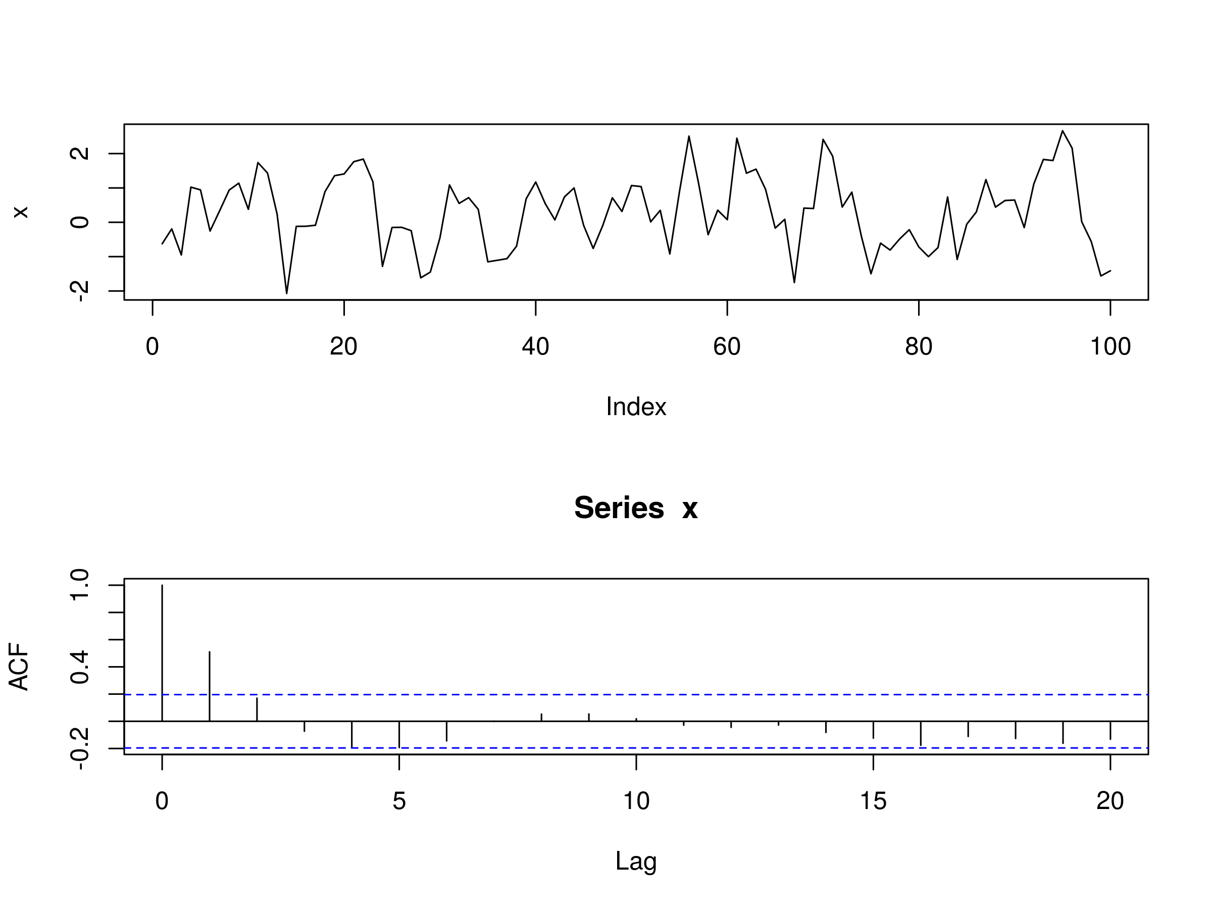 Realisation of AR(1) Model, with $\alpha_1 = 0.6$ and Associated Correlogram
Let's now try fitting an AR(p) process to the simulated data we've just generated, to see if we can recover the underlying parameters. You may recall that we carried out a similar procedure in the article on white noise and random walks.
As it turns out R provides a useful command ar to fit autoregressive models. We can use this method to firstly tell us the best order $p$ of the model (as determined by the AIC above) and provide us with parameter estimates for the $\alpha_i$, which we can then use to form confidence intervals.
For completeness, let's recreate the $x$ series:
> set.seed(1)
> x <- w <- rnorm(100)
> for (t in 2:100) x[t] <- 0.6*x[t-1] + w[t]
Now we use the ar command to fit an autoregressive model to our simulated AR(1) process, using maximum likelihood estimation (MLE) as the fitting procedure.
We will firstly extract the best obtained order:
> x.ar <- ar(x, method = "mle")
> x.ar$order
1
The ar command has successfully determined that our underlying time series model is an AR(1) process.
We can then obtain the $\alpha_i$ parameter(s) estimates:
> x.ar$ar
0.5231187
The MLE procedure has produced an estimate, $\hat{\alpha_1} = 0.523$, which is slightly lower than the true value of $\alpha_1 = 0.6$.
Finally, we can use the standard error (with the asymptotic variance) to construct 95% confidence intervals around the underlying parameter(s). To achieve this, we simply create a vector c(-1.96, 1.96) and then multiply it by the standard error:
x.ar$ar + c(-1.96, 1.96)*sqrt(x.ar$asy.var)
0.3556050 0.6906324
The true parameter does fall within the 95% confidence interval, as we'd expect from the fact we've generated the realisation from the model specifically.
How about if we change the $\alpha_1 =-0.6$?
> set.seed(1)
> x <- w <- rnorm(100)
> for (t in 2:100) x[t] <- -0.6*x[t-1] + w[t]
> layout(1:2)
> plot(x, type="l")
> acf(x)
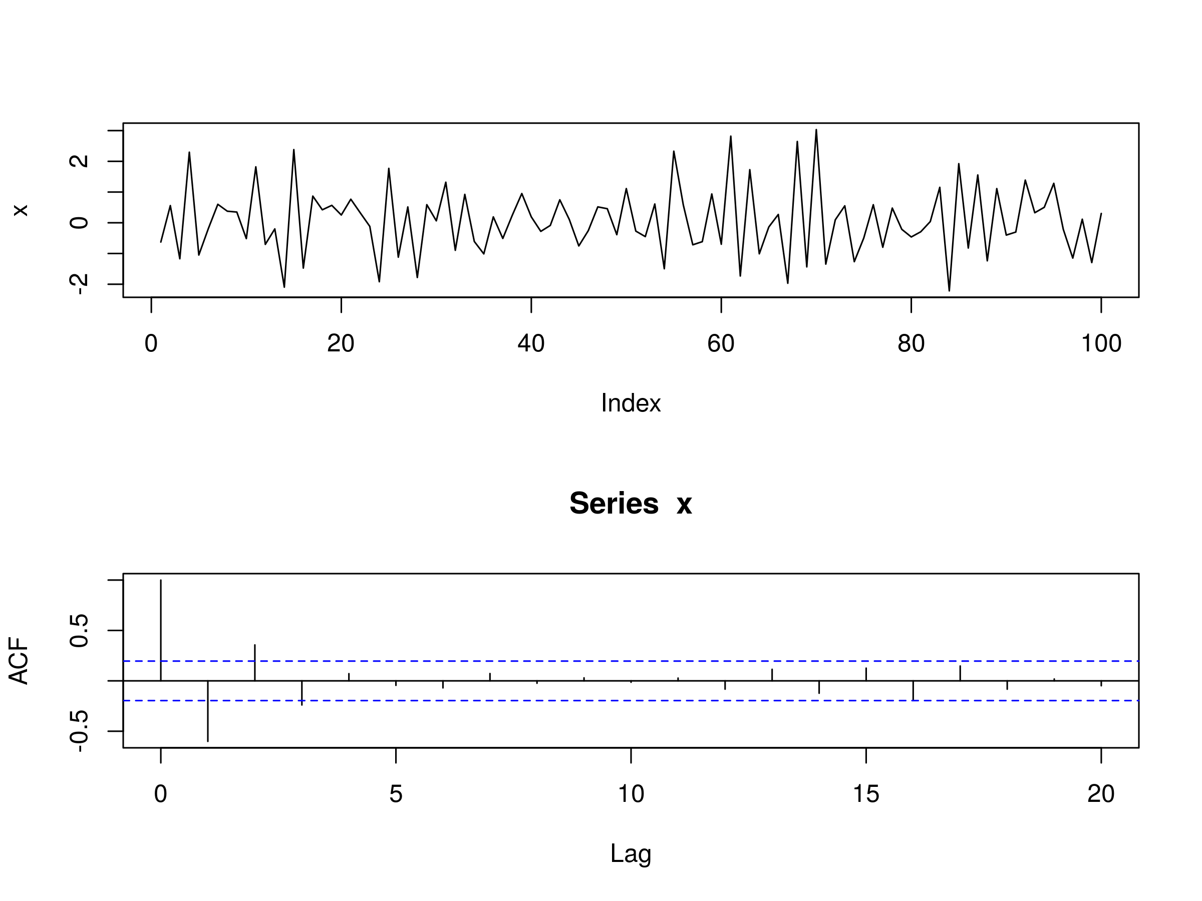 Realisation of AR(1) Model, with $\alpha_1 = -0.6$ and Associated Correlogram
As before we can fit an AR(p) model using ar:
> set.seed(1)
> x <- w <- rnorm(100)
> for (t in 2:100) x[t] <- -0.6*x[t-1] + w[t]
> x.ar <- ar(x, method = "mle")
> x.ar$order
1
> x.ar$ar
-0.5973473
> x.ar$ar + c(-1.96, 1.96)*sqrt(x.ar$asy.var)
-0.7538593 -0.4408353
Once again we recover the correct order of the model, with a very good estimate $\hat{\alpha_1}=-0.597$ of $\alpha_1=-0.6$. We also see that the true parameter falls within the 95% confidence interval once again.
AR(2)
Let's add some more complexity to our autoregressive processes by simulating a model of order 2. In particular, we will set $\alpha_1=0.666$, but also set $\alpha_2 = -0.333$. Here's the full code to simulate and plot the realisation, as well as the correlogram for such a series:
> set.seed(1)
> x <- w <- rnorm(100)
> for (t in 3:100) x[t] <- 0.666*x[t-1] - 0.333*x[t-2] + w[t]
> layout(1:2)
> plot(x, type="l")
> acf(x)
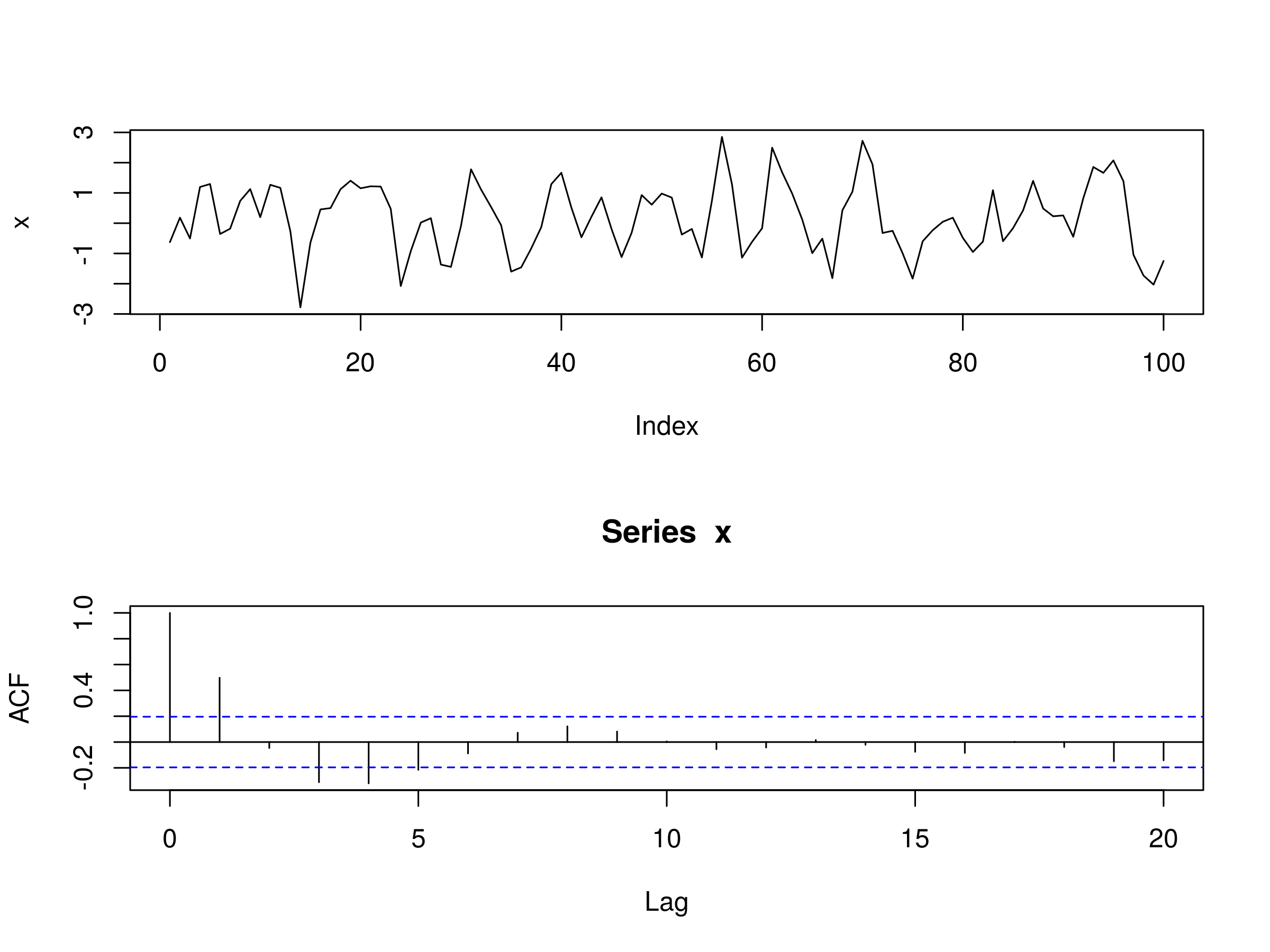 Realisation of AR(2) Model, with $\alpha_1 = 0.666$, $\alpha_2 = -0.333$ and Associated Correlogram
As before we can see that the correlogram differs significantly from that of white noise, as we'd expect. There are statistically significant peaks at $k=1$, $k=3$ and $k=4$.
Once again, we're going to use the ar command to fit an AR(p) model to our underlying AR(2) realisation. The procedure is similar as for the AR(1) fit:
> set.seed(1)
> x <- w <- rnorm(100)
> for (t in 3:100) x[t] <- 0.666*x[t-1] - 0.333*x[t-2] + w[t]
> x.ar <- ar(x, method = "mle")
Warning message:
In arima0(x, order = c(i, 0L, 0L), include.mean = demean) :
  possible convergence problem: optim gave code = 1
> x.ar$order
2
> x.ar$ar
0.6961005 -0.3946280
The correct order has been recovered and the parameter estimates $\hat{\alpha_1}=0.696$ and $\hat{\alpha_2}=-0.395$ are not too far off the true parameter values of $\alpha_1=0.666$ and $\alpha_2=-0.333$.
Notice that we receive a convergence warning message. Notice also that R actually uses the arima0 function to calculate the AR model. As we'll learn in subsequent articles, AR(p) models are simply ARIMA(p, 0, 0) models, and thus an AR model is a special case of ARIMA with no Moving Average (MA) component.
We'll also be using the arima command to create confidence intervals around multiple parameters, which is why we've neglected to do it here.
Now that we've created some simulated data it is time to apply the AR(p) models to financial asset time series.
Financial Data
Amazon Inc.
Let's begin by obtaining the stock price for Amazon (AMZN) using quantmod as in the last article:
> require(quantmod)
> getSymbols("AMZN")
> AMZN
..
..
2015-08-12    523.75    527.50   513.06     525.91     3962300        525.91
2015-08-13    527.37    534.66   525.49     529.66     2887800        529.66
2015-08-14    528.25    534.11   528.25     531.52     1983200        531.52
The first task is to always plot the price for a brief visual inspection. In this case we'll using the daily closing prices:
> plot(Cl(AMZN))
You'll notice that quantmod adds some formatting for us, namely the date, and a slightly prettier chart than the usual R charts:
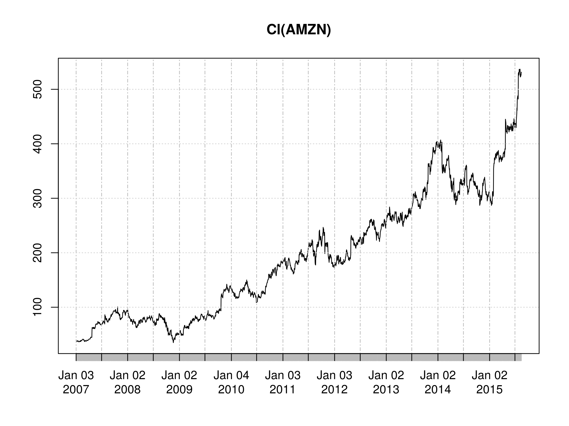 Daily Closing Price of AMZN
We are now going to take the logarithmic returns of AMZN and then the first-order difference of the series in order to convert the original price series from a non-stationary series to a (potentially) stationary one.
This allows us to compare "apples to apples" between equities, indices or any other asset, for use in later multivariate statistics, such as when calculating a covariance matrix. If you would like a detailed explanation as to why log returns are preferable, take a look at this article over at Quantivity.
Let's create a new series, amznrt, to hold our differenced log returns:
> amznrt = diff(log(Cl(AMZN)))
Once again, we can plot the series:
> plot(amznrt)
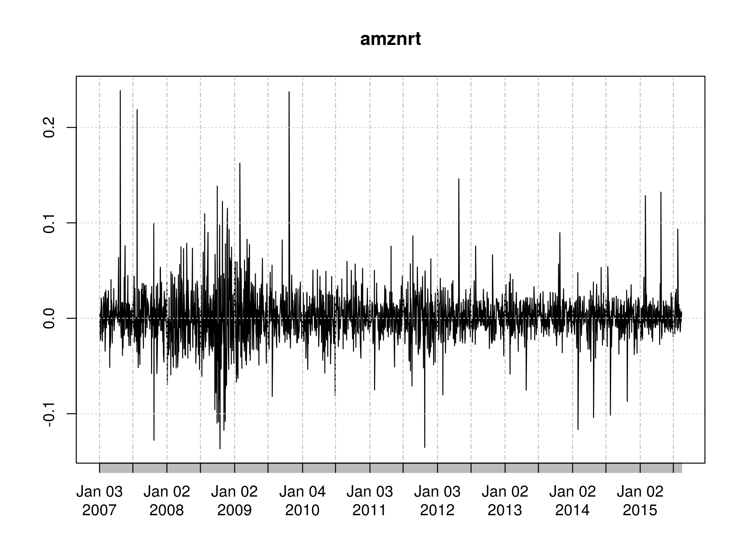 First Order Differenced Daily Logarithmic Returns of AMZN Closing Prices
At this stage we want to plot the correlogram. We're looking to see if the differenced series looks like white noise. If it does not then there is unexplained serial correlation, which might be "explained" by an autoregressive model.
> acf(amznrt, na.action=na.omit)
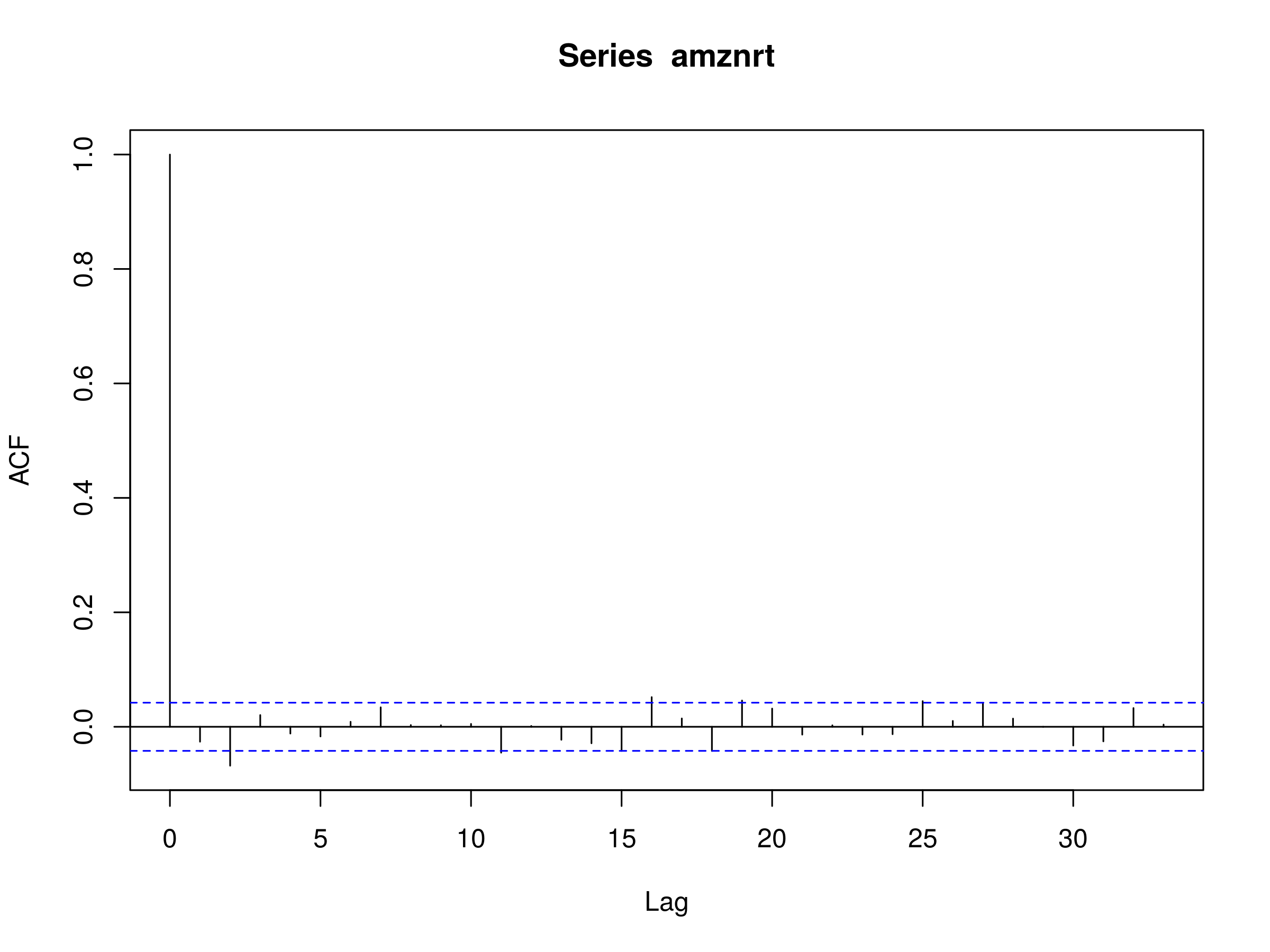 Correlogram of First Order Differenced Daily Logarithmic Returns of AMZN Closing Prices
We notice a statististically significant peak at $k=2$. Hence there is a reasonable possibility of unexplained serial correlation. Be aware though, that this may be due to sampling bias. As such, we can try fitting an AR(p) model to the series and produce confidence intervals for the parameters:
> amznrt.ar <- ar(amznrt, na.action=na.omit)
> amznrt.ar$order
2
> amznrt.ar$ar
-0.02779869 -0.06873949
> amznrt.ar$asy.var
            [,1]        [,2]
[1,] 4.59499e-04 1.19519e-05
[2,] 1.19519e-05 4.59499e-04
Fitting the ar autoregressive model to the first order differenced series of log prices produces an AR(2) model, with $\hat{\alpha_1} = -0.0278$ and $\hat{\alpha_2} = -0.0687$. I've also output the aysmptotic variance so that we can calculate standard errors for the parameters and produce confidence intervals. We want to see whether zero is part of the 95% confidence interval, as if it is, it reduces our confidence that we have a true underlying AR(2) process for the AMZN series.
To calculate the confidence intervals at the 95% level for each parameter, we use the following commands. We take the square root of the first element of the asymptotic variance matrix to produce a standard error, then create confidence intervals by multiplying it by -1.96 and 1.96 respectively, for the 95% level:
> -0.0278 + c(-1.96, 1.96)*sqrt(4.59e-4)
-0.0697916 0.0141916
> -0.0687 + c(-1.96, 1.96)*sqrt(4.59e-4)
-0.1106916 -0.0267084
Note that this becomes more straightforward when using the arima function, but we'll wait until Part 2 before introducing it properly.
Thus we can see that for $\alpha_1$ zero is contained within the confidence interval, while for $\alpha_2$ zero is not contained in the confidence interval. Hence we should be very careful in thinking that we really have an underlying generative AR(2) model for AMZN.
In particular we note that the autoregressive model does not take into account volatility clustering, which leads to clustering of serial correlation in financial time series. When we consider the ARCH and GARCH models in later articles, we will account for this.
When we come to use the full arima function in the next article, we will make predictions of the daily log price series in order to allow us to create trading signals.
S&P500 US Equity Index
Along with individual stocks we can also consider the US Equity index, the S&P500. Let's apply all of the previous commands to this series and produce the plots as before:
> getSymbols("^GSPC")
> GSPC
..
..
2015-08-12   2081.10   2089.06  2052.09    2086.05  4269130000       2086.05
2015-08-13   2086.19   2092.93  2078.26    2083.39  3221300000       2083.39
2015-08-14   2083.15   2092.45  2080.61    2091.54  2795590000       2091.54
We can plot the prices:
> plot(Cl(GSPC))
 Daily Closing Price of S&500
As before, we'll create the first order difference of the log closing prices:
> gspcrt = diff(log(Cl(GSPC)))
Once again, we can plot the series:
> plot(gspcrt)
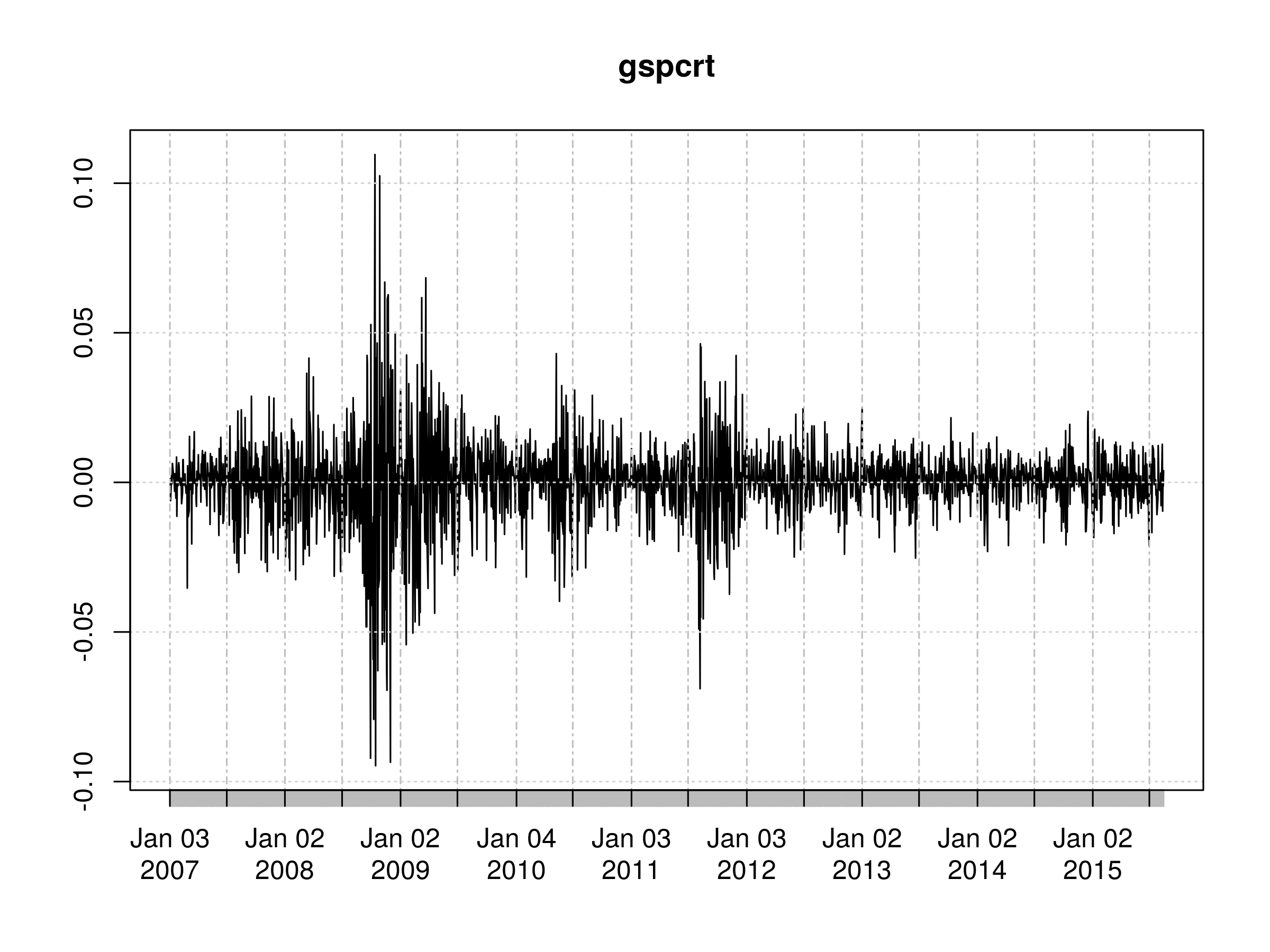 First Order Differenced Daily Logarithmic Returns of S&500 Closing Prices
It is clear from this chart that the volatility is not stationary in time. This is also reflected in the plot of the correlogram. There are many peaks, including $k=1$ and $k=2$, which are statistically significant beyond a white noise model.
In addition, we see evidence of long-memory processes as there are some statistically significant peaks at $k=16$, $k=18$ and $k=21$:
> acf(gspcrt, na.action=na.omit)
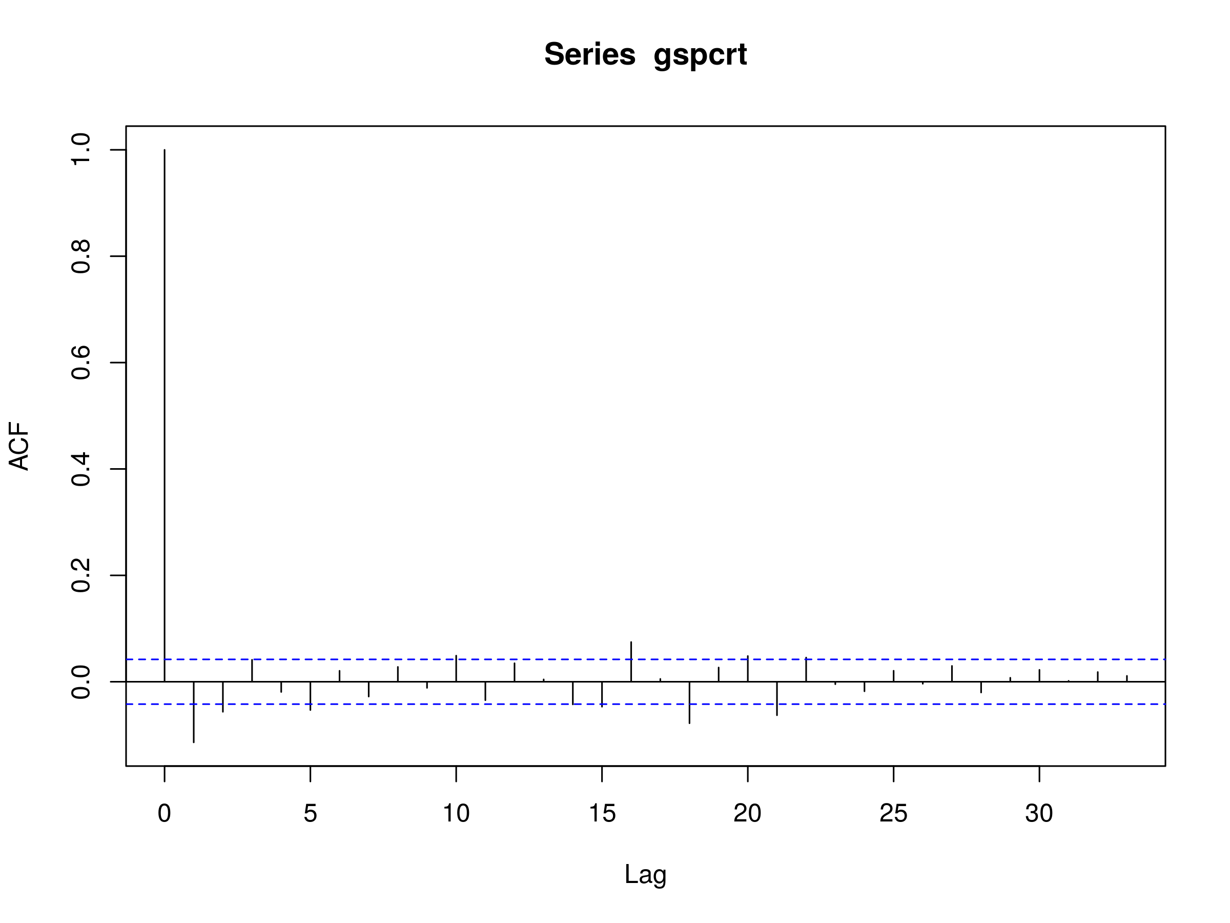 Correlogram of First Order Differenced Daily Logarithmic Returns of S&500 Closing Prices
Ultimately we will need a more sophisticated model than an autoregressive model of order p. However, at this stage we can still try fitting such a model. Let's see what we get if we do so:
> gspcrt.ar <- ar(gspcrt, na.action=na.omit)
> gspcrt.ar$order
22
> gspcrt.ar$ar
 [1] -0.111821507 -0.060150504  0.018791594 -0.025619932 -0.046391435
 [6]  0.002266741 -0.030089046  0.030430265 -0.007623949  0.044260402
[11] -0.018924358  0.032752930 -0.001074949 -0.042891664 -0.039712505
[16]  0.052339497  0.016554471 -0.067496381  0.007070516  0.035721299
[21] -0.035419555  0.031325869
Using ar produces an AR(22) model, i.e. a model with 22 non-zero parameters! What does this tell us? It is indicative that there is likely a lot more complexity in the serial correlation than a simple linear model of past prices can really account for.
However, we already knew this because we can see that there is significant serial correlation in the volatility. For instance, consider the highly volatile period around 2008.
This motivates the next set of models, namely the Moving Average MA(q) and the Autoregressive Moving Average ARMA(p, q). We'll learn about both of these in Part 2 of this article. As we repeatedly mention, these will ultimately lead us to the ARIMA and GARCH family of models, both of which will provide a much better fit to the serial correlation complexity of the S&500.
This will allows us to improve our forecasts significantly and ultimately produce more profitable strategies.


