In this article we are going to consider the famous Generalised Autoregressive Conditional Heteroskedasticity model of order p,q, also known as GARCH(p,q). GARCH is used extensively within the financial industry as many asset prices are conditional heteroskedastic.
We will be discussing conditional heteroskedasticity at length in this article, leading us to our first conditional heteroskedastic model, known as ARCH. Then we will discuss extensions to ARCH, leading us to the GARCH model. We will then apply GARCH to some financial series that exhibit volatility clustering.
Quick Recap and Next Steps
To date we have considered the following models. The links will take you to the appropriate articles. I highly recommend reading the series in order if you have not done so already:
In the previous article on ARIMA we actually carried out some basic forecasting. We mentioned that once we had studied ARIMA and GARCH we would be in a position to make a simple trading strategy. Thus the final piece to the puzzle is to examine conditional heteroskedasticity in detail and then use that to improve our forecasted results.
Volatility
The main motivation for studying conditional heteroskedasticity in finance is that of volatility of asset returns. Volatility is an incredibly important concept in finance because it is highly synonymous with risk.
Volatility has a wide range of applications in finance:
- Options Pricing - The Black-Scholes model for options prices is dependent upon the volatility of the underlying instrument
- Risk Management - Volatility plays a role in calculating the VaR of a portfolio, the Sharpe Ratio for a trading strategy and in determination of leverage
- Tradeable Securities - Volatility can now be traded directly by the introduction of the CBOE Volatility Index (VIX), and subsequent futures contracts and ETFs
Hence, if we can effectively forecast volatility then we will be able to price options more accurately, create more sophisticated risk management tools for our algorithmic trading portfolios and even come up with new strategies that trade volatility directly.
We're now going to turn our attention to conditional heteroskedasticity and discuss what it means.
Conditional Heteroskedasticity
Let's first discuss the concept of heteroskedasticity and then examine the "conditional" part.
If we have a collection of random variables, such as elements in a time series model, we say that the collection is heteroskedastic if there are certain groups, or subsets, of variables within the larger set that have a different variance from the remaining variables.
For instance, in a non-stationary time series that exhibits seasonality or trending effects, we may find that the variance of the series increases with the seasonality or the trend. This form of regular variability is known as heteroskedasticity.
However, in finance there are many reasons why an increase in variance is correlated to a further increase in variance.
For instance, consider the prevalence of downside portfolio protection insurance employed by long-only fund managers. If the equities markets were to have a particularly challenging day (i.e. a substantial drop!) it could trigger automated risk management sell orders, which would further depress the price of equities within these portfolios. Since the larger portfolios are generally highly correlated anyway, this could trigger significant downward volatility.
These "sell-off" periods, as well as many other forms of volatility that occur in finance, lead to heteroskedasticity that is serially correlated and hence conditional on periods of increased variance. Thus we say that such series are conditional heteroskedastic.
One of the challenging aspects of conditional heteroskedastic series is that if we were to plot the correlogram of a series with volatility we might still see what appears to be a realisation of stationary discrete white noise. That is, the volatility itself is hard to detect purely from the correlogram. This is despite the fact that the series is most definitely non-stationary as its variance is not constant in time.
We are going to describe a mechanism for detecting conditional heteroskedastic series in this article and then use the ARCH and GARCH models to account for it, ultimately leading to more realistic forecasting performance, and thus more profitable trading strategies.
Autoregressive Conditional Heteroskedastic Models
We've now discussed conditional heteroskedasticity (CH) and its importance within financial series. We now want a model that can incorporate CH in a natural way. We know that the ARIMA class of models does not account for CH, so how can we proceed?
Well, how about a model that utilises an autoregressive process for the variance itself? That is, a model that actually accounts for the changes in the variance over time using past values of the variance.
This is the basis of the Autoregressive Conditional Heteroskedastic (ARCH) model. We'll begin with the simplest possible case, namely an ARCH model that depends solely on the previous variance value in the series.
Definition
Autoregressive Conditional Heteroskedastic Model of Order Unity
A time series $\{ \epsilon_t \}$ is given at each instance by: \begin{eqnarray} \epsilon_t = \sigma_t w_t \end{eqnarray}
Where $\{ w_t \}$ is discrete white noise, with zero mean and unit variance, and $\sigma^2_t$ is given by:
\begin{eqnarray} \sigma^2_t = \alpha_0 + \alpha_1 \epsilon^2_{t-1} \end{eqnarray}Where $\alpha_0$ and $\alpha_1$ are parameters of the model.
We say that $\{ \epsilon_t \}$ is an autoregressive conditional heteroskedastic model of order unity, denoted by ARCH(1). Substituting for $\sigma^2_t$, we receive:
\begin{eqnarray} \epsilon_t = w_t \sqrt{\alpha_0 + \alpha_1 \epsilon_{t-1}^2} \end{eqnarray}Why Does This Model Volatility?
I personally find the above "formal" definition lacking in motivation as to how it introduces volatility. However, you can see how it is introduced by squaring both sides of the previous equation:
\begin{eqnarray} \operatorname{Var}(\epsilon_t) &=& \operatorname{E}[\epsilon^2_t ] - (\operatorname{E}[\epsilon_t ])^2 \\ &=& \operatorname{E}[\epsilon^2_t ] \\ &=& \operatorname{E}[w^2_t ] \operatorname{E}[\alpha_0 + \alpha_1 \epsilon^2_{t-1} ] \\ &=& \operatorname{E}[\alpha_0 + \alpha_1 \epsilon^2_{t-1} ] \\ &=& \alpha_0 + \alpha_1 \operatorname{Var}(\epsilon_{t-1}) \end{eqnarray}Where I have used the definitions of the variance $\operatorname{Var}(x) = \operatorname{E}[x^2] - (\operatorname{E}[x])^2$ and the linearity of the expectation operator $\operatorname{E}$, along with the fact that $\{w_t \}$ has zero mean and unit variance.
Thus we can see that the variance of the series is simply a linear combination of the variance of the prior element of the series. Simply put, the variance of an ARCH(1) process follows an AR(1) process.
It is interesting to compare the ARCH(1) model with an AR(1) model. Recall that the latter is given by:
\begin{eqnarray} x_t = \alpha_0 + \alpha_1 x_{t-1} + w_t \end{eqnarray}You can see that the models are similar in form (with the exception of the white noise term).
When Is It Appropriate To Apply ARCH(1)?
So what approach can we take in order to determine whether an ARCH(1) model is appropriate to apply to a series?
Consider that when we were attempting to fit an AR(1) model we were concerned with the decay of the first lag on a correlogram of the series.
However, if we apply the same logic to the square of the residuals, and see whether we can apply an AR(1) to these square residuals then we have an indication that an ARCH(1) process may be appropriate.
Note that ARCH(1) should only ever be applied to a series that has already had an appropriate model fitted sufficient to leave the residuals looking like discrete white noise. Since we can only tell whether ARCH is appropriate or not by squaring the residuals and examining the correlogram, we also need to ensure that the mean of the residuals is zero.
Crucially, ARCH should only ever be applied to series that do not have any trends or seasonal effects, i.e. that has no (evident) serially correlation. ARIMA is often applied to such a series (or even Seasonal ARIMA), at which point ARCH may be a good fit.
ARCH(p) Models
It is straightforward to extend ARCH to higher order lags. An ARCH(p) process is given by:
\begin{eqnarray} \epsilon_t = w_t \sqrt{\alpha_0 + \sum^p_{i=1} \alpha_p \epsilon^2_{t-i}} \end{eqnarray}You can think of ARCH(p) as applying an AR(p) model to the variance of the series.
An obvious question to ask at this stage is if we are going to apply an AR(p) process to the variance, why not a Moving Average MA(q) model as well? Or a mixed model such as ARMA(p,q)?
This is actually the motivation for the Generalised ARCH model, known as GARCH, which we will now define and discuss.
Generalised Autoregressive Conditional Heteroskedastic Models
Definition
Generalised Autoregressive Conditional Heteroskedastic Model of Order p, q
A time series $\{ \epsilon_t \}$ is given at each instance by: \begin{eqnarray} \epsilon_t = \sigma_t w_t \end{eqnarray}
Where $\{ w_t \}$ is discrete white noise, with zero mean and unit variance, and $\sigma^2_t$ is given by:
\begin{eqnarray} \sigma^2_t = \alpha_0 + \sum^{q}_{i=1} \alpha_i \epsilon^2_{t-i} + \sum^{p}_{j=1} \beta_j \sigma^2_{t-j} \end{eqnarray}Where $\alpha_i$ and $\beta_j$ are parameters of the model.
We say that $\{ \epsilon_t \}$ is a generalised autoregressive conditional heteroskedastic model of order p,q, denoted by GARCH(p,q).
Hence this definition is similar to that of ARCH(p), with the exception that we are adding moving average terms, that is the value of $\sigma^2$ at $t$, $\sigma^2_t$, is dependent upon previous $\sigma^2_{t-j}$ values.
Thus GARCH is the "ARMA equivalent" of ARCH, which only has an autoregressive component.
Simulations, Correlograms and Model Fittings
As always we're going to begin with the simplest possible case of the model, namely GARCH(1,1). This means we are going to consider a single autoregressive lag and a single "moving average" lag. The model is given by the following:
\begin{eqnarray} \epsilon_t &=& \sigma_t w_t \\ \sigma^2_t &=& \alpha_0 + \alpha_1 \epsilon^2_{t-1} + \beta_1 \sigma^2_{t-1} \end{eqnarray}Note that it is necessary for $\alpha_1 + \beta_1 < 1$ otherwise the series will become unstable.
We can see that the model has three parameters, namely $\alpha_0$, $\alpha_1$ and $\beta_1$. Let's set $\alpha_0 = 0.2$, $\alpha_1=0.5$ and $\beta_1=0.3$.
To create the GARCH(1,1) model in R we need to perform a similar procedure as for our original random walk simulations. That is, we need to create a vector w to store our random white noise values, then a separate vector eps to store our time series values and finally a vector sigsq to store the ARMA variances.
We can use the R rep command to create a vector of zeros that we will populate with our GARCH values:
> set.seed(2)
> a0 <- 0.2
> a1 <- 0.5
> b1 <- 0.3
> w <- rnorm(10000)
> eps <- rep(0, 10000)
> sigsq <- rep(0, 10000)
> for (i in 2:10000) {
>   sigsq[i] <- a0 + a1 * (eps[i-1]^2) + b1 * sigsq[i-1]
>   eps[i] <- w[i]*sqrt(sigsq[i])
> }
At this stage we have generated our GARCH model using the aforementioned parameters over 10,000 samples. We are now in a position to plot the correlogram:
> acf(eps)
Notice that the series look like a realisation of a discrete white noise process:
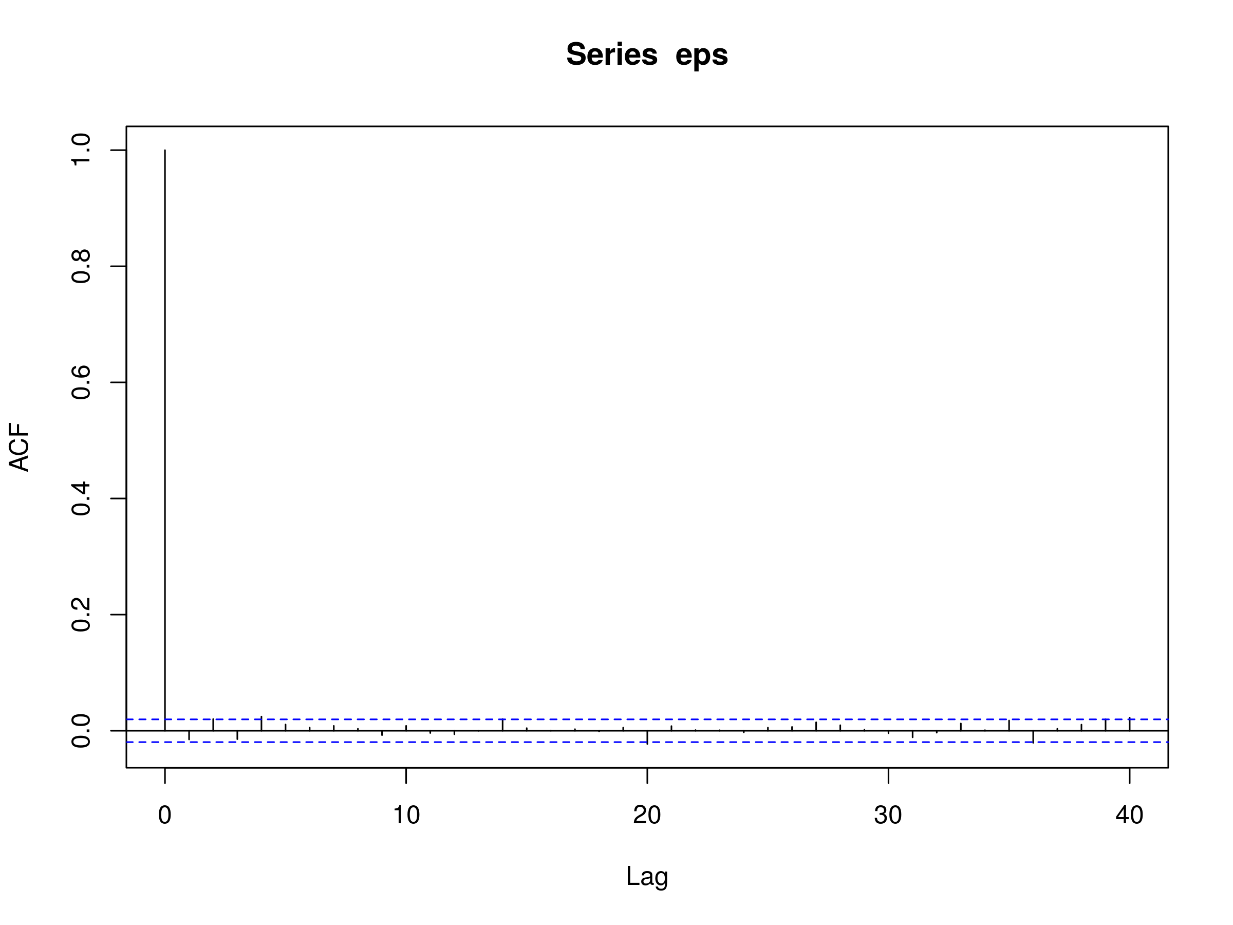 Correlogram of a simulated GARCH(1,1) model with $\alpha_0=0.2$, $\alpha_1=0.5$ and $\beta_1=0.3$
However, if we plot correlogram of the square of the series:
> acf(eps^2)
We see substantial evidence of a conditionally heteroskedastic process via the decay of successive lags:
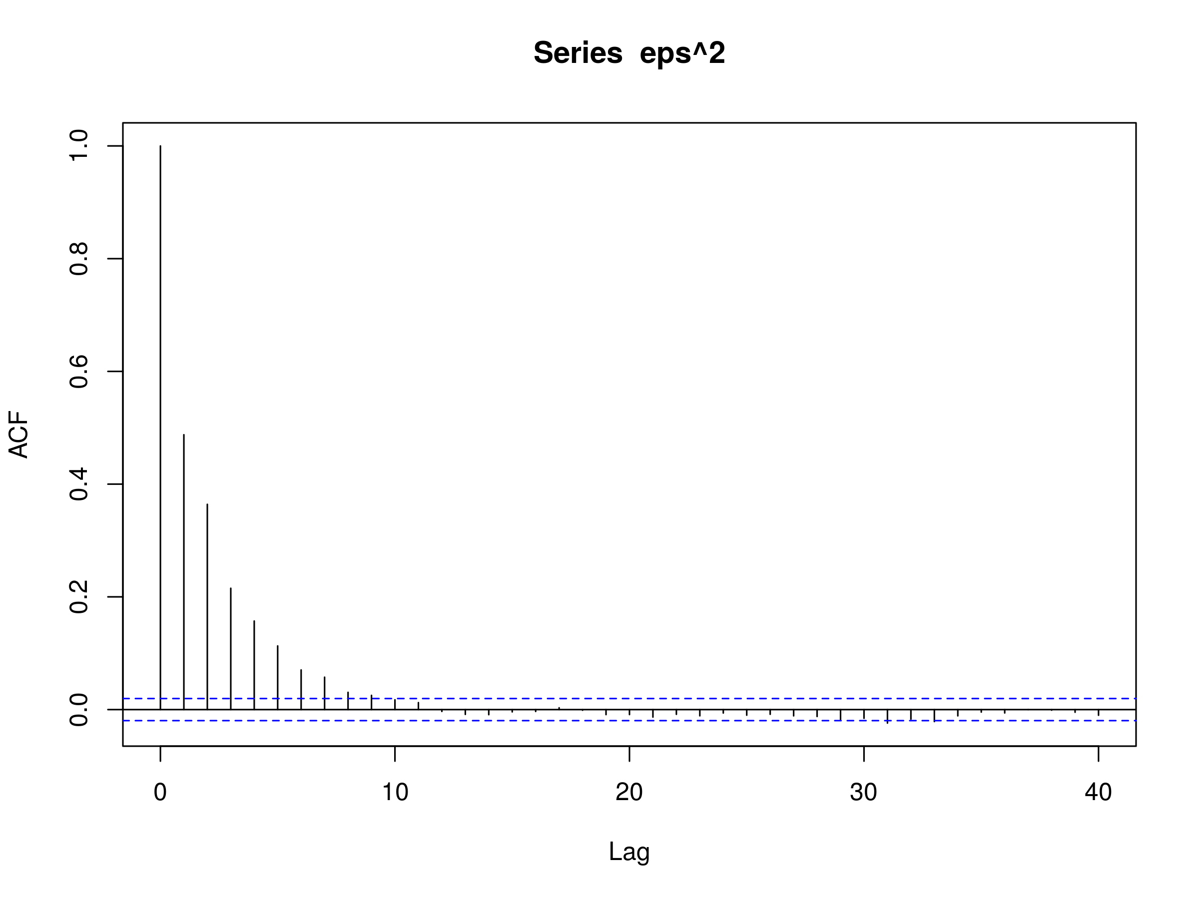 Correlogram of a simulated GARCH(1,1) models squared values with $\alpha_0=0.2$, $\alpha_1=0.5$ and $\beta_1=0.3$
As in the previous articles we now want to try and fit a GARCH model to this simulated series to see if we can recover the parameters. Thankfully, a helpful library called tseries provides the garch command to carry this procedure out:
> require(tseries)
We can then use the confint command to produce confidence intervals at the 97.5% level for the parameters:
> eps.garch <- garch(eps, trace=FALSE)
> confint(eps.garch)
       2.5 %    97.5 %
a0 0.1786255 0.2172683
a1 0.4271900 0.5044903
b1 0.2861566 0.3602687
We can see that the true parameters all fall within the respective confidence intervals.
Financial Data
Now that we know how to simulate and fit a GARCH model, we want to apply the procedure to some financial series. In particular, let's try fitting ARIMA and GARCH to the FTSE 100 index of the largest UK companies by market capitalisation. Yahoo Finance uses the symbol "^FTSE" for the index. We can use quantmod to obtain the data:
> require(quantmod)
> getSymbols("^FTSE")
We can then calculate the differences of the log returns of the closing price:
> ftrt = diff(log(Cl(FTSE)))
Let's plot the values:
> plot(ftrt)
It is very clear that there are periods of significant increases in volatility, particularly around 2008-2009, late 2011 and more recently in mid 2015:
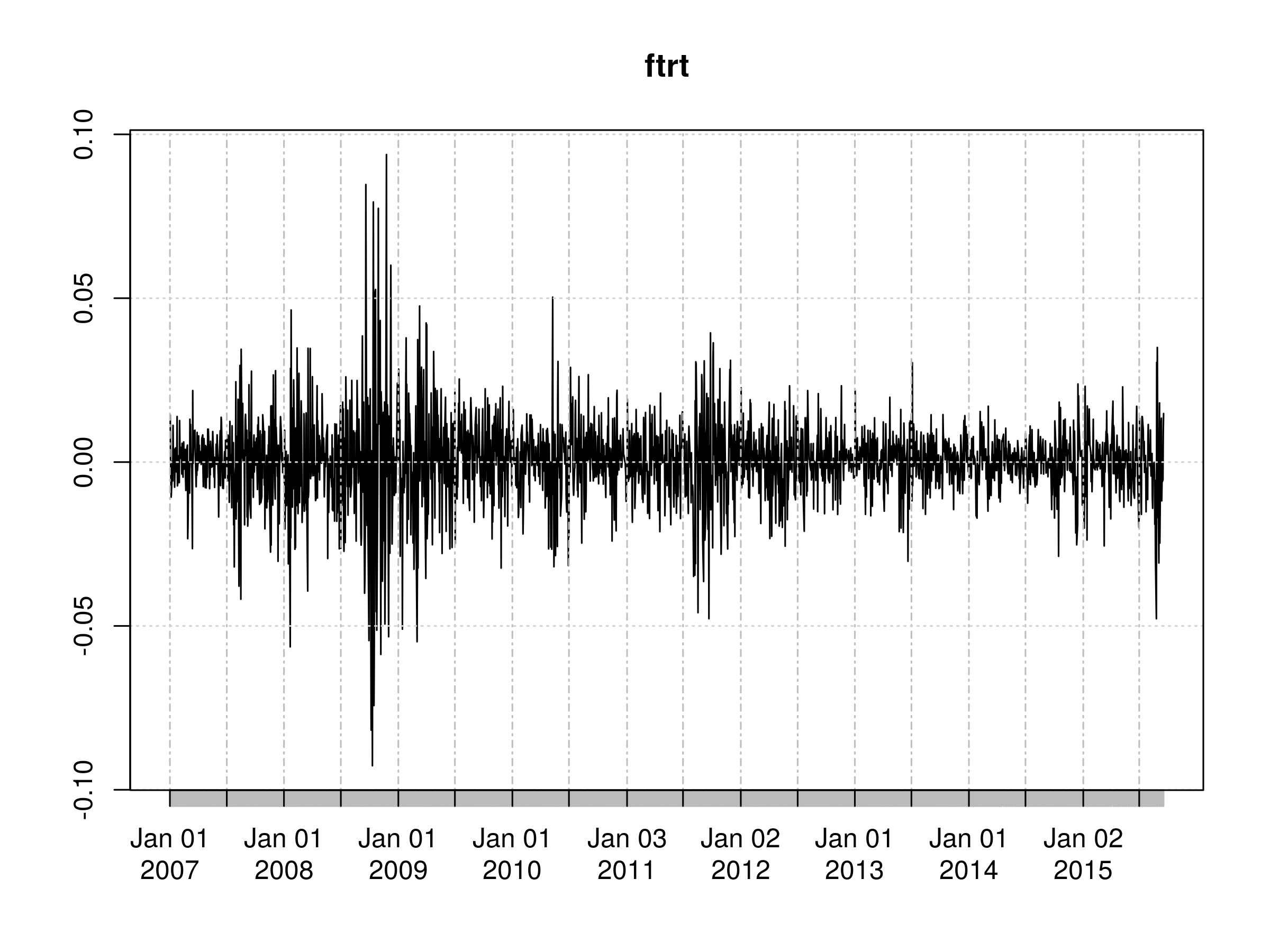 Differenced log returns of the daily closing price of the FTSE 100 UK stock index
We also need to remove the NA value generated by the differencing procedure:
> ft <- as.numeric(ftrt)
> ft <- ft[!is.na(ft)]
The next task is to fit a suitable ARIMA(p,d,q) model. We saw how to do that in the previous article, so I won't repeat the procedure here, I will simply provide the code:
> ftfinal.aic <- Inf
> ftfinal.order <- c(0,0,0)
> for (p in 1:4) for (d in 0:1) for (q in 1:4) {
>   ftcurrent.aic <- AIC(arima(ft, order=c(p, d, q)))
>   if (ftcurrent.aic < ftfinal.aic) {
>     ftfinal.aic <- ftcurrent.aic
>     ftfinal.order <- c(p, d, q)
>     ftfinal.arima <- arima(ft, order=ftfinal.order)
>   }
> }
Since we've already differenced the FTSE returns once, we should expect our integrated component $d$ to equal zero, which it does:
> ftfinal.order
[1] 4 0 4
Thus we receive an ARIMA(4,0,4) model, that is four autoregressive parameters and four moving average parameters.
We are now in a position to decide whether the residuals of this model fit possess evidence of conditional heteroskedastic behaviour. To test this we need to plot the correlogram of the residuals:
> acf(resid(ftfinal.arima))
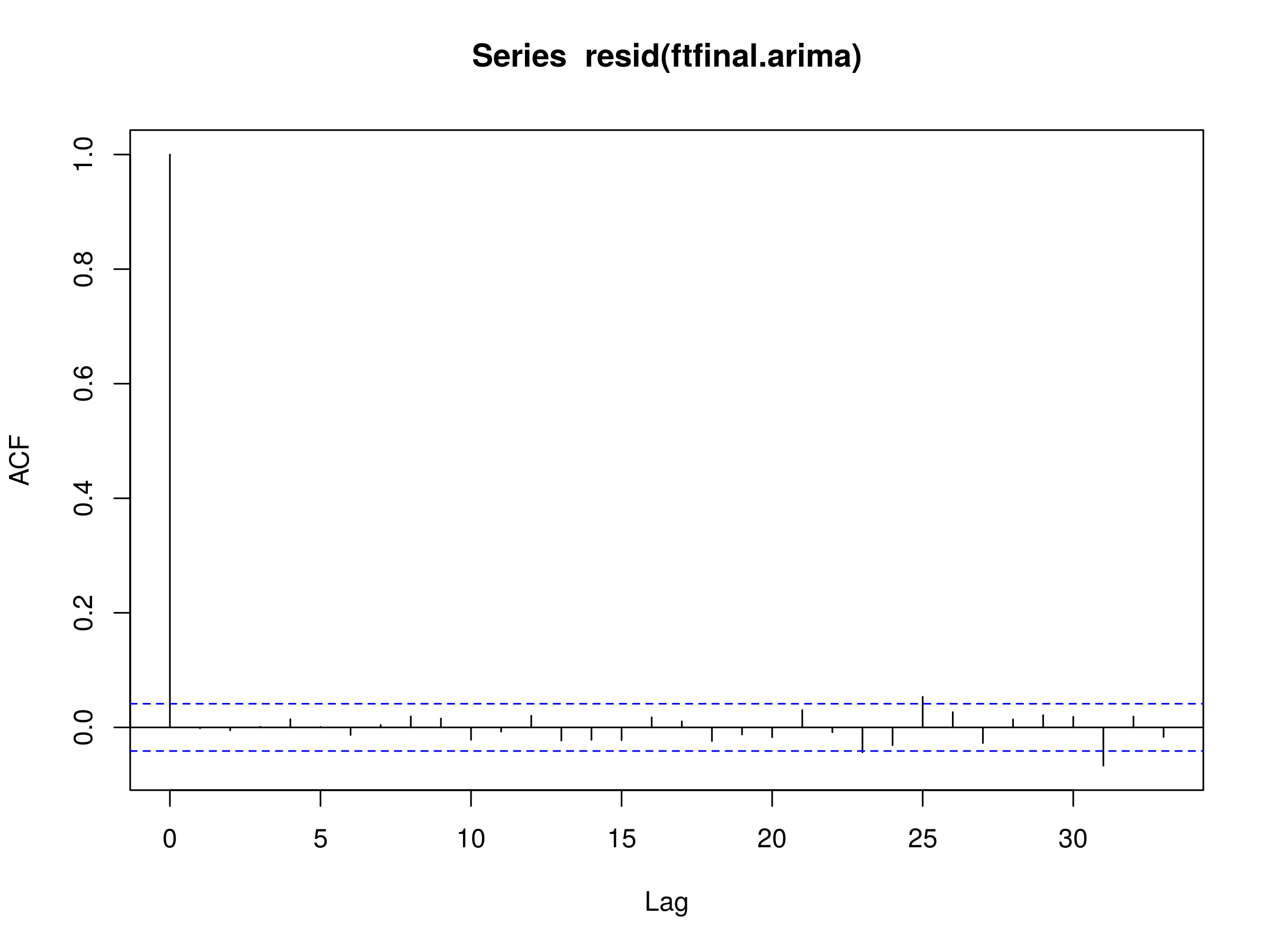 Residuals of an ARIMA(4,0,4) fit to the FTSE100 diff log returns
This looks like a realisation of a discrete white noise process indicating that we have achieved a good fit with the ARIMA(4,0,4) model.
To test for conditional heteroskedastic behaviour we need to square the residuals and plot the corresponding correlogram:
> acf(resid(ftfinal.arima)^2)
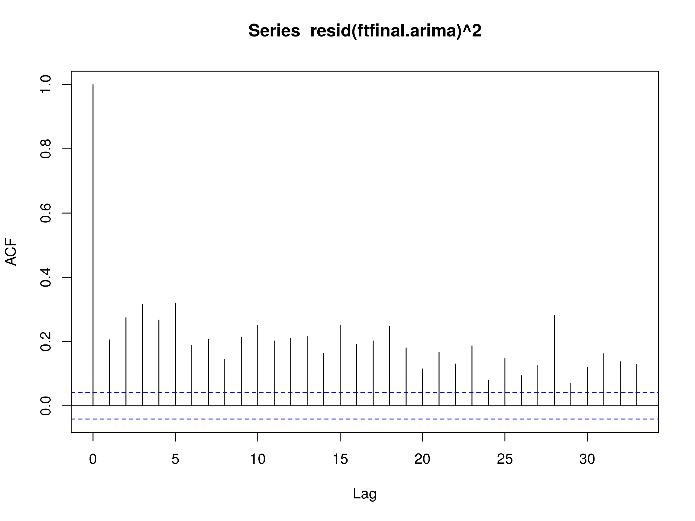 Squared residuals of an ARIMA(4,0,4) fit to the FTSE100 diff log returns
We can see clear evidence of serial correlation in the squared residuals, leading us to the conclusion that conditional heteroskedastic behaviour is present in the diff log return series of the FTSE100.
We are now in a position to fit a GARCH model using the tseries library.
The first command actually fits an appropriate GARCH model, with the trace=F parameter telling R to suppress excessive output.
The second command removes the first element of the residuals, since it is NA:
> ft.garch <- garch(ft, trace=F)
> ft.res <- ft.garch$res[-1]
Finally, to test for a good fit we can plot the correlogram of the GARCH residuals and the square GARCH residuals:
> acf(ft.res)
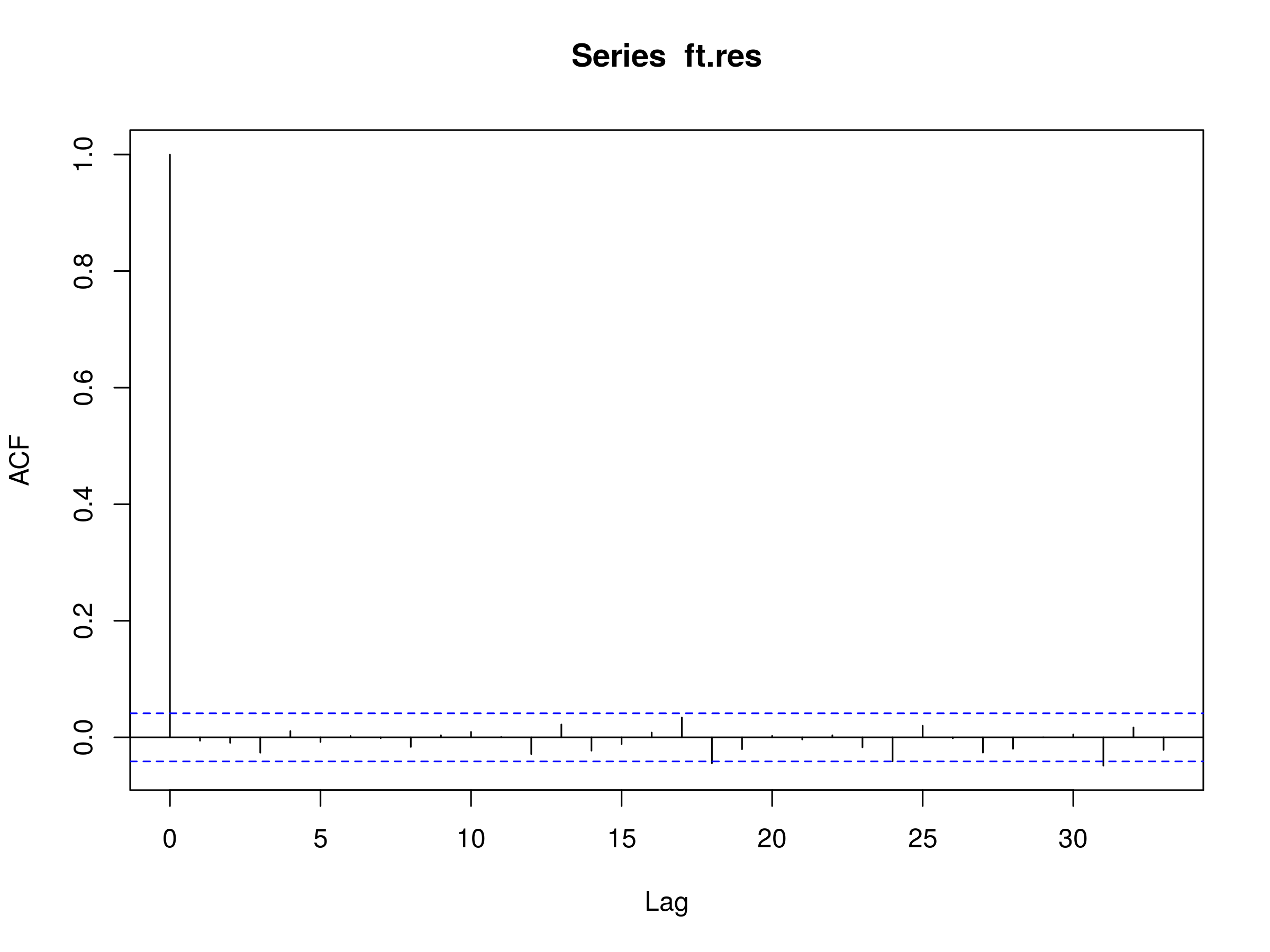 Residuals of a GARCH(p,q) fit to the ARIMA(4,0,4) fit of the FTSE100 diff log returns
The correlogram looks like a realisation of a discrete white noise process, indicating a good fit. Let's now try the squared residuals:
> acf(ft.res^2)
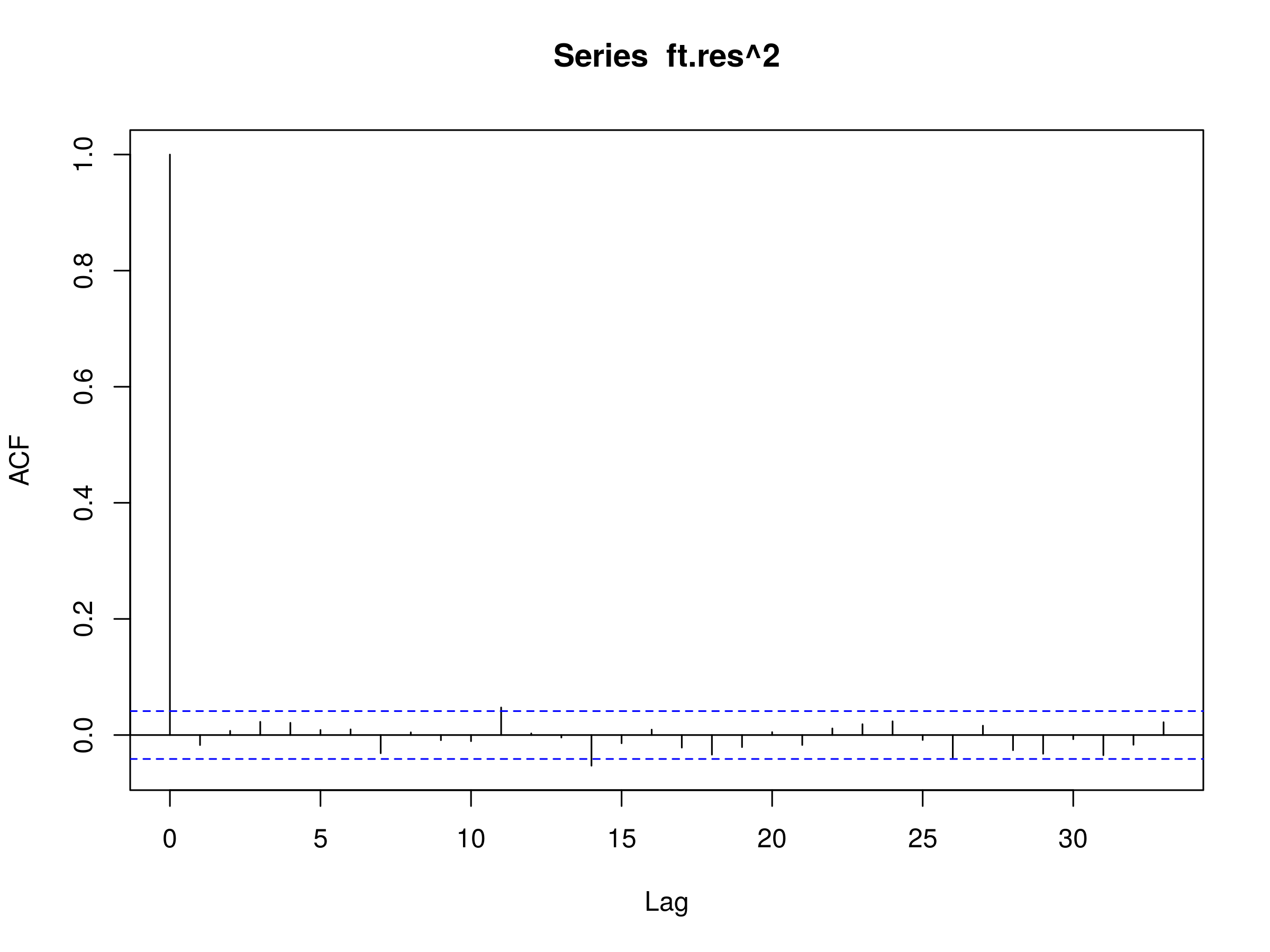 Squared residuals of a GARCH(p,q) fit to the ARIMA(4,0,4) fit of the FTSE100 diff log returns
Once again, we have what looks like a realisation of a discrete white noise process, indicating that we have "explained" the serial correlation present in the squared residuals with an appropriate mixture of ARIMA(p,d,q) and GARCH(p,q).
Next Steps
We are now at the point in our time series education where we have studied ARIMA and GARCH, allowing us to fit a combination of these models to a stock market index, and to determine if we have achieved a good fit or not.
The next step is to actually produce forecasts of future daily returns values from this combination and use it to create a basic trading strategy. That will be the subject of the next article.


