Dynamic Hedge Ratio Between ETF Pairs Using the Kalman Filter

A common quant trading technique involves taking two assets that form a cointegrating relationship and utilising a mean-reverting approach to construct a trading strategy. This can be carried out by performing a linear regression between the two assets (such as a pair of ETFs) and using this to determine how much of each asset to long and short at particular thresholds.

One of the major concerns with such a strategy is that any parameters introduced via this structural relationship, such as the hedging ratio between the two assets, are likely to be time-varying. That is, they are not fixed throughout the period of the strategy. In order to improve profitability it would be useful if we could determine a mechanism for adjusting the hedging ratio over time.

One approach to this problem is to utilise a rolling linear regression with a lookback window. This involves updating the linear regression on every bar so that the slope and intercept terms "follow" the latest behaviour of the cointegration relationship. However it also introduces another free parameter into the strategy, namely the lookback window length. This must be optimised, often via cross-validation.

A more sophisticated approach is to utilise a state space model that treats the "true" hedge ratio as an unobserved hidden variable and attempts to estimate it with "noisy" observations. In our case this means the pricing data of each asset.

The Kalman Filter performs exactly this task. In a previous article we had an in-depth look at the Kalman Filter and how it could be viewed as a Bayesian updating process.

In this article we are going to make use of the Kalman Filter, via the pykalman Python library, to help us dynamically estimate the slope and intercept (and hence hedging ratio) between a pair of ETFs.

This technique will ultimately be backtested with the new QSTrader open-source trading system, which will enable us to see how performance of such a strategy has changed in the last few years.

The plots in this post were largely inspired by, and extended from a post written by Aidan O'Mahoney, who runs The Algo Engineer blog.

Brief Recap of the Kalman Filter

If you want to read a more mathematically in-depth article about the Kalman Filter, please take a look at the previous article. I'll briefly recap the key points here.

The state space model we are going to use consists of two matrix equations. The first is known as the state or transition equation and describes how a set of state variables, $\theta_t$ are changed from one time period to the next. There is a linear dependence on the previous state given by the transition matrix $G_t$ as well as a normally-distributed system noise $w_t$. Note that $G=G_t$, which in the general sense means that the transition matrix is itself time dependent:

\begin{eqnarray} \theta_t = G_t \theta_{t-1} + w_t \end{eqnarray}

However, these states are often unobservable and we might only get access to observations at each time index, which are given by $y_t$. The observations also have an associated observation equation which includes a linear component via the observation matrix $F_t$, as well as a measurement noise, also normally distributed, given by $v_t$:

\begin{eqnarray} y_t = F_t \theta_t + v_t \end{eqnarray}

For more details on the state space model and the Kalman Filter please refer to my previous article.

Incorporating Linear Regression into a Kalman Filter

The main question at this stage is how do we utilise this state space model to incorporate the information in a linear regression?

If we recall from the previous article on the MLE for linear regression we know that a multiple linear regression states that a response value $y$ is a linear function of its feature inputs ${\bf x}$:

\begin{eqnarray} y({\bf x}) = \beta^T {\bf x} + \epsilon \end{eqnarray}

Where $\beta^T = (\beta_0, \beta_1, \ldots, \beta_p)$ represents the transpose vector of the intercept $\beta_0$ and slopes $\beta_i$, with $\epsilon \sim \mathcal{N}(\mu, \sigma^2)$ represents the error term.

Since we are in a one-dimensional setting we can simply write $\beta^T = (\beta_0, \beta_1)$ and ${\bf x} = \begin{pmatrix} 1 \\ x \end{pmatrix}$.

We set the (hidden) states of our system to be given by the vector $\beta^T$, that is the intercept and slope of our linear regression. The next step is to assume that tomorrow's intercept and slope are equal to today's intercept and slope with the addition of some random system noise. This gives it the nature of a random walk, the behaviour of which is discussed at length in the previous article on white noise and random walks:

\begin{eqnarray} \beta_{t+1} ={\bf I} \beta_{t} + w_t \end{eqnarray}

Where the transition matrix is set to the two-dimensional indentify matrix, $G_t = {\bf I}$. This is one half of the state space model. The next step is to actually use one of the ETFs in the pair as the "observations".

Applying the Kalman Filter to a Pair of ETFs

To form the observation equation it is necessary to choose one of the ETF pricing series to be the "observed" variables, $y_t$, and the other to be given by $x_t$, which provides the linear regression formulation as above:

\begin{eqnarray} y_t &=& F_t {\bf x}_t + v_t \\ &=& (\beta_0, \beta_1 ) \begin{pmatrix} 1 \\ x_t \end{pmatrix} + v_t \end{eqnarray}

Thus we have the linear regression reformulated as a state space model, which allows us to estimate the intercept and slope as new price points arrive via the Kalman Filter.

TLT and ETF

We are going to consider two fixed income ETFs, namely the iShares 20+ Year Treasury Bond ETF (TLT) and the iShares 3-7 Year Treasury Bond ETF (IEI). Both of these ETFs track the performance of varying duration US Treasury bonds and as such are both exposed to similar market factors. We will analyse their regression behaviour over the last five years or so.

Scatterplot of ETF Prices

We are now going to use a variety of Python libraries, including numpy, matplotlib, pandas and pykalman to to analyse the behaviour of a dynamic linear regression between these two securities. As with all Python programs the first task is to import the necessary libraries:

from __future__ import print_function

import matplotlib.pyplot as plt
import numpy as np
import pandas as pd
from pandas.io.data import DataReader
from pykalman import KalmanFilter

Note: You will likely need to run pip install pykalman to install the PyKalman library.

The next step is write the function draw_date_coloured_scatterplot to produce a scatterplot of the asset adjusted closing prices (such a scatterplot is inspired by that produced by Aidan O'Mahony). The scatterplot will be coloured using a matplotlib colour map, specifically "Yellow To Red", where yellow represents price pairs closer to 2010, while red represents price pairs closer to 2016:

def draw_date_coloured_scatterplot(etfs, prices):
    """
    Create a scatterplot of the two ETF prices, which is
    coloured by the date of the price to indicate the 
    changing relationship between the sets of prices    
    """
    # Create a yellow-to-red colourmap where yellow indicates
    # early dates and red indicates later dates
    plen = len(prices)
    colour_map = plt.cm.get_cmap('YlOrRd')    
    colours = np.linspace(0.1, 1, plen)
    
    # Create the scatterplot object
    scatterplot = plt.scatter(
        prices[etfs[0]], prices[etfs[1]], 
        s=30, c=colours, cmap=colour_map, 
        edgecolor='k', alpha=0.8
    )
    
    # Add a colour bar for the date colouring and set the 
    # corresponding axis tick labels to equal string-formatted dates
    colourbar = plt.colorbar(scatterplot)
    colourbar.ax.set_yticklabels(
        [str(p.date()) for p in prices[::plen//9].index]
    )
    plt.xlabel(prices.columns[0])
    plt.ylabel(prices.columns[1])
    plt.show()

I've commented the code so it should be fairly straightforward to see what all of the commands are doing. The main work is being done within the colour_map, colours and scatterplot variables. It produces the following plot:

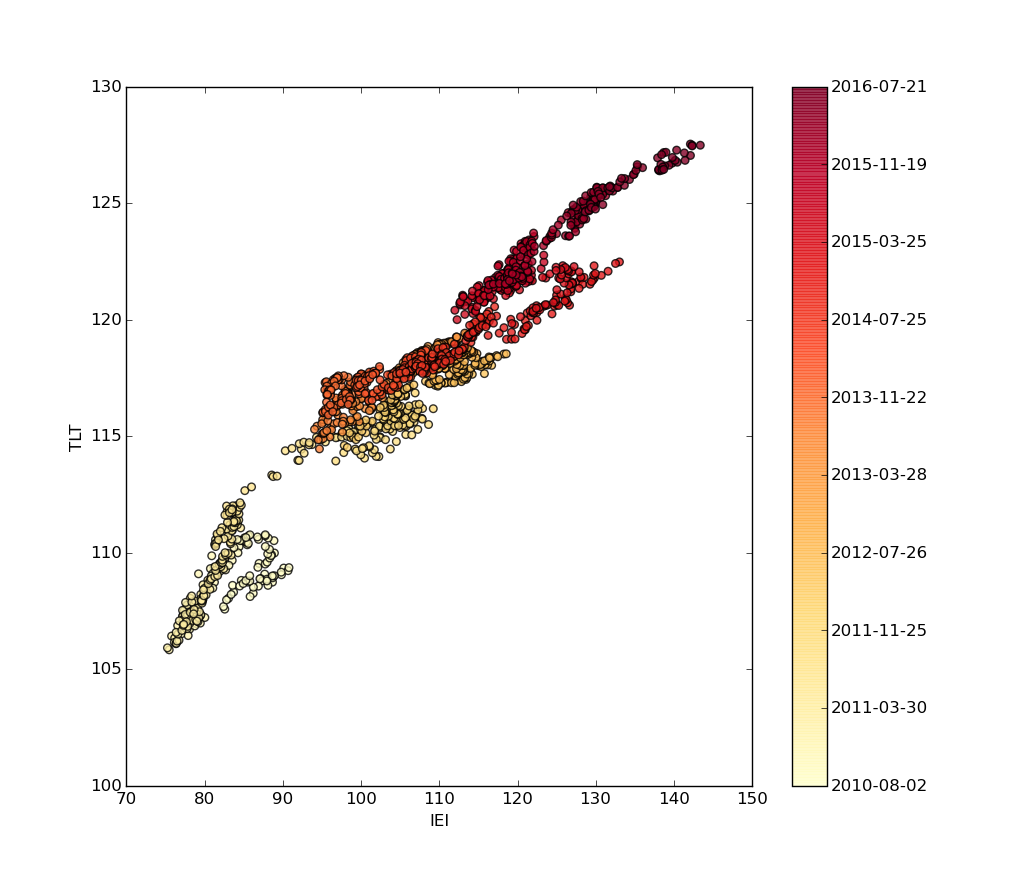Scatterplot of the fixed income ETFs, TFT vs IEI

Time-Varying Slope and Intercept

The next step is to actually use pykalman to dynamically adjust the intercept and slope between TFT and IEI. This function is more complex and requires some explanation.

Firstly we define a variable called delta, which is used to control the transition covariance for the system noise. In my original article on the Kalman Filter this was denoted by $W_t$. We simply multiply such a value by the two-dimensional identity matrix.

The next step is to create the observation matrix. As we previously described this matrix is a row vector consisting of the prices of TFT and a sequence of unity values. To construct this we utilise the numpy vstack method to vertically stack these two price series into a single column vector, which we then transpose.

At this point we use the KalmanFilter class from pykalman to create the Kalman Filter instance. We supply it with the dimensionality of the observations (unity in this case), the dimensionality of the states (two in this case as we are looking at the intercept and slope in the linear regression).

We also need to supply the mean and covariance of the initial state. In this instance we set the initial state mean to be zero for both intercept and slope, while we take the two-dimensional identity matrix for the initial state covariance. The transition matrices are also given by the two-dimensional identity matrix.

The last terms to specify are the observation matrices as above in obs_mat, with its covariance equal to unity. Finally the transition covariance matrix (controlled by delta) is given by trans_cov, described above.

Now that we have the kf Kalman Filter instance we can use it to filter based on the adjusted prices from IEI. This provides us with the state means of the intercept and slope, which is what we're after. In addition we also receive the covariances of the states.

This is all wrapped up in the calc_slope_intercept_kalman function:

def calc_slope_intercept_kalman(etfs, prices):
    """
    Utilise the Kalman Filter from the pyKalman package
    to calculate the slope and intercept of the regressed
    ETF prices.
    """
    delta = 1e-5
    trans_cov = delta / (1 - delta) * np.eye(2)
    obs_mat = np.vstack(
        [prices[etfs[0]], np.ones(prices[etfs[0]].shape)]
    ).T[:, np.newaxis]
    
    kf = KalmanFilter(
        n_dim_obs=1, 
        n_dim_state=2,
        initial_state_mean=np.zeros(2),
        initial_state_covariance=np.ones((2, 2)),
        transition_matrices=np.eye(2),
        observation_matrices=obs_mat,
        observation_covariance=1.0,
        transition_covariance=trans_cov
    )
    
    state_means, state_covs = kf.filter(prices[etfs[1]].values)
    return state_means, state_covs

Finally we plot these values as returned from the previous function. To achieve this we simply create a pandas DataFrame of the slopes and intercepts at time values $t$, using the index from the prices DataFrame, and plot each column as a subplot:

def draw_slope_intercept_changes(prices, state_means):
    """
    Plot the slope and intercept changes from the 
    Kalman Filte calculated values.
    """
    pd.DataFrame(
        dict(
            slope=state_means[:, 0], 
            intercept=state_means[:, 1]
        ), index=prices.index
    ).plot(subplots=True)
    plt.show()

The output is given as follows:

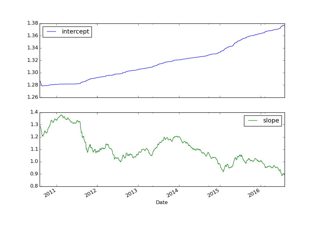Time-varying slope and intercept of a linear regression between ETFs TFT and IEI

Clearly the time-varying slope changes dramatically over the 2011 to 2016 period, dropping from around 1.38 in 2011 to around 0.9 in 2016. It is not difficult to see that utilising a fixed hedge ratio in a pairs trading strategy would be far too rigid.

In addition the estimate of the slope is relatively noisy. This can be controlled by the delta variable given in the code above but has the effect of also reducing the responsiveness of the filter to changes in the "true" unobserved hedge ratio between the two ETFs.

When we come to develop a trading strategy it will be necessary to optimise this parameter delta across baskets of pairs of ETFs utilising cross-validation once again.

Next Steps

Now that we've been able to construct a dynamic hedging ratio between the two ETFs, we need a way to actually carry out a trading strategy based off of this information. The next article in the series will make use of QSTrader to perform a backtest on various pairs in order to see how performance changes when parameters and time periods are varied.

Bibliographic Note

Utilising the Kalman Filter for "online linear regression" has been carried out by many quant trading individuals. Ernie Chan utilises the technique in his book^[1] to estimate the dynamic linear regression coefficients between the two ETFs: EWA and EWC.

Aidan O'Mahony used matplotlib and pykalman to also estimate the regression coefficients in his post^[2], which inspired the diagrams for this current article.

Jonathan Kinlay discusses the application of the Kalman Filter to simulated financial data^[3] and suggests that it might be advisable to use the KF to suppress trade signals generated at in periods of high noise, or increase allocations to pairs where the noise is low.

An introductory discussion about the Kalman Filter, using the R programming language, can be found in Cowpertwait and Metcalfe^[4].

References

Full Code

from __future__ import print_function

import matplotlib.pyplot as plt
import numpy as np
import pandas as pd
from pandas.io.data import DataReader
from pykalman import KalmanFilter


def draw_date_coloured_scatterplot(etfs, prices):
    """
    Create a scatterplot of the two ETF prices, which is
    coloured by the date of the price to indicate the 
    changing relationship between the sets of prices    
    """
    # Create a yellow-to-red colourmap where yellow indicates
    # early dates and red indicates later dates
    plen = len(prices)
    colour_map = plt.cm.get_cmap('YlOrRd')    
    colours = np.linspace(0.1, 1, plen)
    
    # Create the scatterplot object
    scatterplot = plt.scatter(
        prices[etfs[0]], prices[etfs[1]], 
        s=30, c=colours, cmap=colour_map, 
        edgecolor='k', alpha=0.8
    )
    
    # Add a colour bar for the date colouring and set the 
    # corresponding axis tick labels to equal string-formatted dates
    colourbar = plt.colorbar(scatterplot)
    colourbar.ax.set_yticklabels(
        [str(p.date()) for p in prices[::plen//9].index]
    )
    plt.xlabel(prices.columns[0])
    plt.ylabel(prices.columns[1])
    plt.show()


def calc_slope_intercept_kalman(etfs, prices):
    """
    Utilise the Kalman Filter from the pyKalman package
    to calculate the slope and intercept of the regressed
    ETF prices.
    """
    delta = 1e-5
    trans_cov = delta / (1 - delta) * np.eye(2)
    obs_mat = np.vstack(
        [prices[etfs[0]], np.ones(prices[etfs[0]].shape)]
    ).T[:, np.newaxis]
    
    kf = KalmanFilter(
        n_dim_obs=1, 
        n_dim_state=2,
        initial_state_mean=np.zeros(2),
        initial_state_covariance=np.ones((2, 2)),
        transition_matrices=np.eye(2),
        observation_matrices=obs_mat,
        observation_covariance=1.0,
        transition_covariance=trans_cov
    )
    
    state_means, state_covs = kf.filter(prices[etfs[1]].values)
    return state_means, state_covs    
    

def draw_slope_intercept_changes(prices, state_means):
    """
    Plot the slope and intercept changes from the 
    Kalman Filte calculated values.
    """
    pd.DataFrame(
        dict(
            slope=state_means[:, 0], 
            intercept=state_means[:, 1]
        ), index=prices.index
    ).plot(subplots=True)
    plt.show()


if __name__ == "__main__":
    # Choose the ETF symbols to work with along with 
    # start and end dates for the price histories
    etfs = ['TLT', 'IEI']
    start_date = "2010-8-01"
    end_date = "2016-08-01"    
    
    # Obtain the adjusted closin prices from Yahoo finance
    prices = DataReader(
        etfs, 'yahoo', start_date, end_date
    )['Adj Close']

    draw_date_coloured_scatterplot(etfs, prices)
    state_means, state_covs = calc_slope_intercept_kalman(etfs, prices)
    draw_slope_intercept_changes(prices, state_means)

References

- [1] Chan, E.P. (2013). Algorithmic Trading: Winning Strategies and Their Rationale.
- [2] O'Mahony, A. (2014). Online Linear Regression using a Kalman Filter
- [3] Kinlay, J. (2015). Statistical Arbitrage Using the Kalman Filter
- [4] Cowpertwait, P.S.P. and Metcalfe, A.V. (2009). Introductory Time Series with R.
- [5] Pole, A., West, M., and Harrison, J. (1994). Applied Bayesian Forecasting.