A while back we considered a trading model based on the application of the ARIMA and GARCH time series models to daily S&P500 data. We mentioned in that article as well as other previous time series analysis articles that we would eventually be considering mean reverting trading strategies and how to construct them.
In this article I want to discuss a topic called cointegration, which is a time series concept that allows us to determine if we are able to form a mean reverting pair of assets. We will cover the time series theory related to cointegration here and in the next article we will show how to apply that to real trading strategies using the new open source backtesting framework: QSTrader.
We will proceed by discussing mean reversion in the traditional "pairs trading" framework. This will lead us to the concept of stationarity of a linear combination of assets, ultimately leading us to cointegration and unit root tests. Once we have outlined these tests we will simulate various time series in the R statistical environment and apply the tests in order to assess cointegration.
Mean Reversion Trading Strategies
The traditional idea of a mean reverting "pairs trade" is to simultaneously long and short two separate assets sharing underlying factors that affect their movements. An example from the equities world might be to long McDonald's (NYSE:MCD) and short Burger King (NYSE:BKW - prior to the merger with Tim Horton's).
The rationale for this is that their long term share prices are likely to be in equilibrium due to the broad market factors affecting hamburger production and consumption. A short-term disruption to an individual in the pair, such as a supply chain disruption solely affecting McDonald's, would lead to a temporary dislocation in their relative prices. This means that a long-short trade carried out at this disruption point should become profitable as the two stocks return to their equilibrium value once the disruption is resolved. This is the essence of the classic "pairs trade".
As quants we are interested in carrying out mean reversion trading not solely on a pair of assets, but also baskets of assets that are separately interrelated.
To achieve this we need a robust mathematical framework for identifying pairs or baskets of assets that mean revert in the manner described above. This is where the concept of cointegrated time series arises.
The idea is to consider a pair of non-stationary time series, such as the random-walk like assets of MCD and BKW, and form a linear combination of each series to produce a stationary series, which has a fixed mean and variance.
This stationary series may have short term disruptions where the value wanders far from the mean, but due to its stationarity this value will eventually return to the mean. Trading strategies can make use of this by longing/shorting the pair at the appropriate disruption point and betting on a longer-term reversion of the series to its mean.
Mean reverting strategies such as this permit a wide range of instruments to create the "synthetic" stationary time series. We are certainly not restricted to "vanilla" equities. For instance, we can make use of Exchange Traded Funds (ETF) that track commodity prices, such as crude oil, and baskets of oil producing companies. Hence there is plenty of scope for identifying such mean reverting systems.
Before we delve into the mechanics of the actual trading strategies, which will be the subject of the next article, we must first understand how to statistically identify such cointegrated series. For this we will utilise techniques from time series analysis, continuing the usage of the R statistical language as in previous articles on the topic.
Cointegration
Now that we've motivated the necessity for a quantitative framework to carry out mean reversion trading we can define the concept of cointegration. Consider a pair of time series, both of which are non-stationary. If we take a particular linear combination of theses series it can sometimes lead to a stationary series. Such a pair of series would then be termed cointegrated.
The mathematical definition is given by:
Cointegration
Let $\{x_t \}$ and $\{y_t \}$ be two non-stationary time series, with $a, b \in \mathbb{R}$, constants. If the combined series $a x_t + b y_t$ is stationary then we say that $\{x_t \}$ and $\{y_t \}$ are cointegrated.
While the definition is useful it does not directly provide us with a mechanism for either determining the values of $a$ and $b$, nor whether such a combination is in fact statistically stationary. For the latter we need to utilise tests for unit roots.
Unit Root Tests
In our previous discussion of autoregressive AR(p) models we explained the role of the characteristic equation. We noted that it was simply an autoregressive model, written in backward shift form, set to equal zero. Solving this equation gave us a set of roots.
In order for the model to be considered stationary all of the roots of the equation had to exceed unity. An AR(p) model with a root equal to unity - a unit root - is non-stationary. Random walks are AR(1) processes with unit roots and hence they are also non-stationary.
Thus in order to detect whether a time series is stationary or not we can construct a statistical hypothesis test for the presence of a unit root in a time series sample.
We are going to consider three separate tests for unit roots: Augmented Dickey-Fuller (AFD), Phillips-Perron and Phillips-Ouliaris. We will see that they are based on differing assumptions but are all ultimately testing for the same issue, namely stationarity of the tested time series sample.
Let's now take a brief look at all three tests in turn.
Augmented Dickey-Fuller Test
Dickey and Fuller[2] were responsible for introducing the following test for the presence of a unit root. The original test considers a time series $z_t = \alpha z_{t-1} + w_t$, in which $w_t$ is discrete white noise. The null hypothesis is that $\alpha = 1$, while the alternative hypothesis is that $\alpha < 1$.
Said and Dickey[6] improved the original Dickey-Fuller test leading to the Augmented Dickey-Fuller (ADF) test, in which the series $z_t$ is modified to an AR(p) model from an AR(1) model. I've discussed the test in a previous article where we've used Python to calculate it. In this article we will carry out the same test using R.
Phillips-Perron Test
The ADF test assumes an AR(p) model as an approximation for the time series sample and uses this to account for higher order autocorrelations. The Phillips-Perron test[5] does not assume an AR(p) model approximation. Instead a non-parametric kernel smoothing method is utilised on the stationary process $w_t$, which allows it to account for unspecified autocorrelation and heteroscedasticity.
Phillips-Ouliaris Test
The Phillips-Ouliaris test[4] is different from the previous two tests in that it is testing for evidence of cointegration among the residuals between two time series. The main idea here is that tests such as ADF, when applied to the estimated cointegrating residuals, do not have the Dickey-Fuller distributions under the null hypothesis where cointegration isn't present. Instead, these distributions are known as Phillips-Ouliaris distributions and hence this test is more appropriate.
Difficulties with Unit Root Tests
While the ADF and Phillips-Perron test are equivalent asymptotically they can produce very different answers in finite samples[7]. This is because they handle autocorrelation and heteroscedasticity differently. It is necessary to be very clear which hypotheses are being tested for when applying these tests and not to simply apply them blindly to arbitrary series.
In addition unit root tests are not great at distinguishing highly persistent stationary processes from non-stationary processes. One must be very careful when using these on certain forms of financial time series. This can be especially problematic when the underlying relationship being modelled (i.e. mean reversion of two similar pairs) naturally breaks down due to regime change or other structural changes in the financial markets.
Simulated Cointegrated Time Series with R
Let's now apply the previous unit root tests to some simulated data that we know to be cointegrated. We can make use of the defiition of cointegration to artificially create two non-stationary time series that share an underlying stochastic trend, but with a linear combination that is stationary.
Our first task is to define a random walk $z_t = z_{t-1} + w_t$, where $w_t$ is discrete white noise. Take a look at the previous article on white noise and random walks if you need to brush up on these concepts.
With the random walk $z_t$ let's create two new time series $x_t$ and $y_t$ that both share the underlying stochastic trend from $z_t$, albeit by different amounts:
\begin{eqnarray} x_t &=& p z_t + w_{x,t} \\ y_t &=& q z_t + w_{y,t} \end{eqnarray}
If we then take a linear combination $a x_t + b y_t$:
\begin{eqnarray} a x_t + b y_t &=& a (p z_t + w_{x,t}) + b (q z_t + w_{y,t}) \\ &=& (ap + bq) z_t + a w_{x,t} + b w_{y,t} \end{eqnarray}
We see that we only achieve a stationary series (that is a combination of white noise terms) if $ap + bq = 0$. We can put some numbers to this to make it more concrete. Suppose $p=0.3$ and $q=0.6$. After some simple algebra we see that if $a=2$ and $b=-1$ we have that $ap +bq = 0$, leading to a stationary series combination. Hence $x_t$ and $y_t$ are cointegrated when $a=2$ and $b=-1$.
Let's simulate this in R in order to visualise the stationary combination. Firstly, we wish to create and plot the underlying random walk series, $z_t$:
set.seed(123)
z <- rep(0, 1000)
for (i in 2:1000) z[i] <- z[i-1] + rnorm(1)
plot(z, type="l")
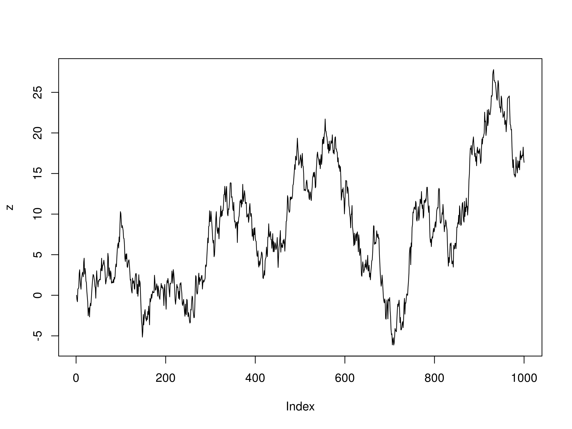 Realisation of a random walk, $z_t$
If we plot both the correlogram of the series and its differences we can see little evidence of autocorrelation:
layout(1:2)
acf(z)
acf(diff(z))
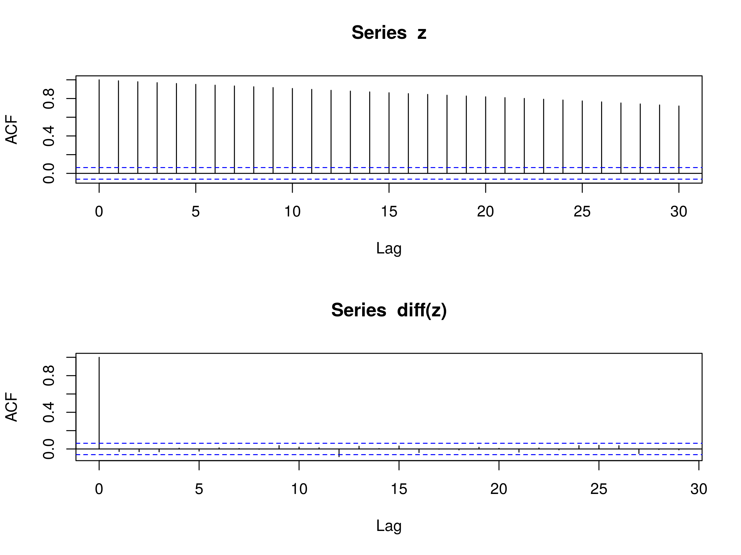 Correlograms of $z_t$ and the differenced series of $z_t$
Hence this realisation of $z_t$ clearly looks like a random walk. The next step is to create $x_t$ and $y_t$ from $z_t$, using $p=0.3$ and $q=0.6$, and then plot both:
x <- y <- rep(0, 1000)
x <- 0.3*z + rnorm(1000)
y <- 0.6*z + rnorm(1000)
layout(1:2)
plot(x, type="l")
plot(y, type="l")
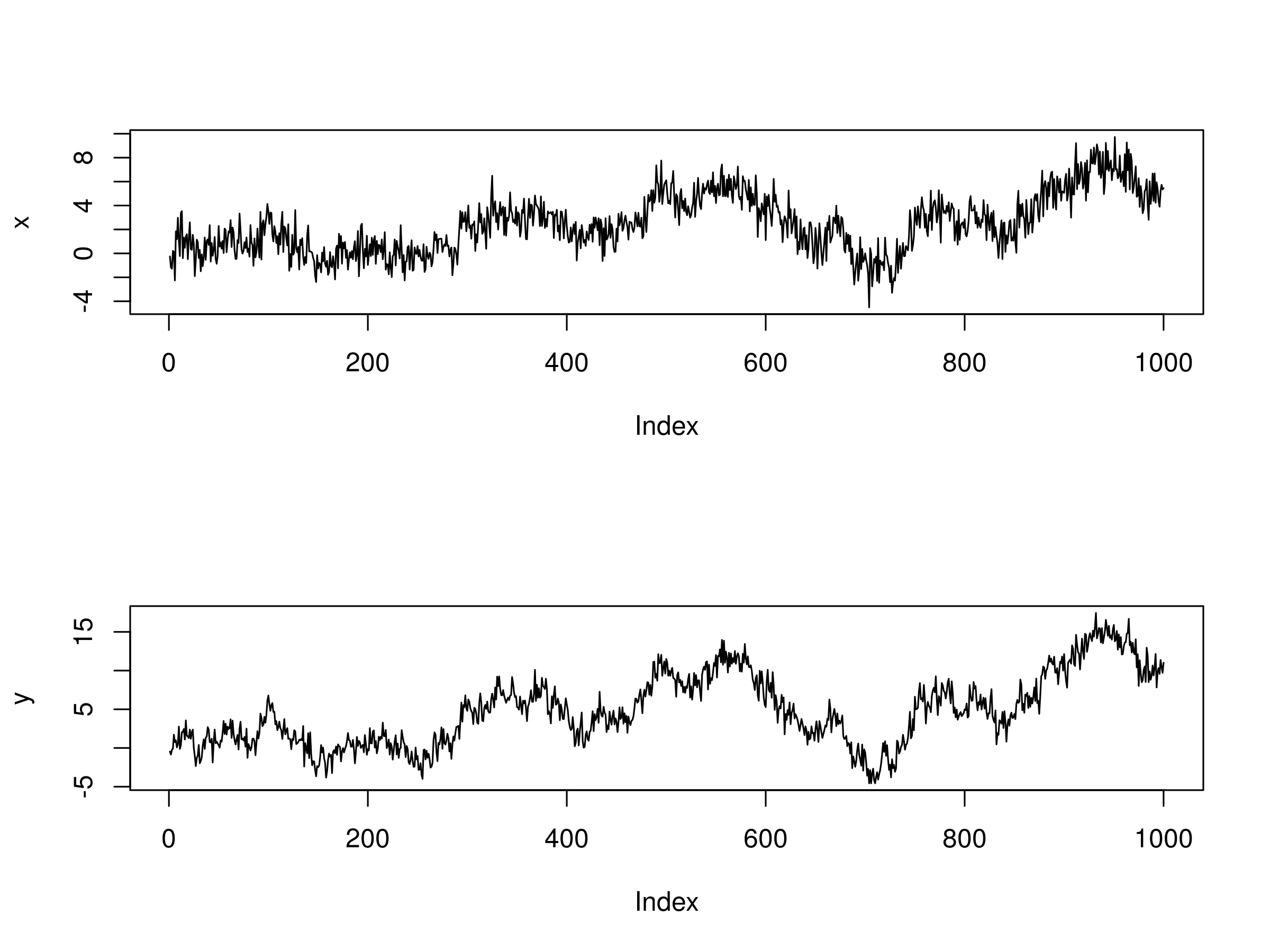 Plot of $x_t$ and $y_t$ series, each based on underlying random walk $z_t$
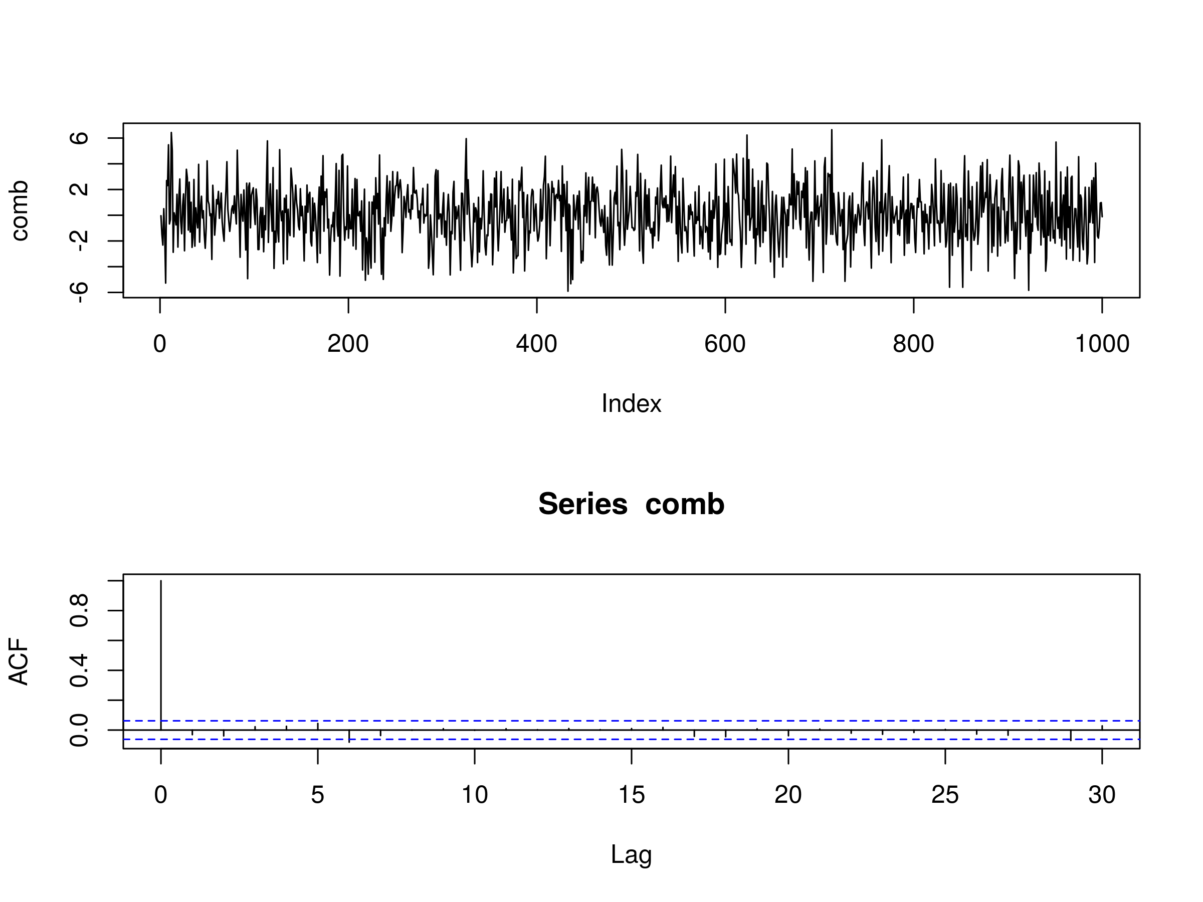
As you can see they both look similar. Of course they will be by definition - they share the same underlying random walk structure from $z_t$. Let's now form the linear combination, comb, using $p=2$ and $q=-1$ and examine the autocorrelation structure:
comb <- 2*x - y
layout(1:2)
plot(comb, type="l")
acf(comb)
 Plot of
 comb - the linear combination series - and its correlogram
It is clear that the combination series comb looks very much like a stationary series. This is to be expected given its definition.
Let's try applying the three unit root tests to the linear combination series. Firstly, the Augmented Dickey-Fuller test:
adf.test(comb)
The output is as follows:
    Augmented Dickey-Fuller Test

data:  comb
Dickey-Fuller = -10.321, Lag order = 9, p-value = 0.01
alternative hypothesis: stationary

Warning message:
In adf.test(comb) : p-value smaller than printed p-value
The p-value is small and hence we have evidence to reject the null hypothesis that the series possesses a unit root. Now we try the Phillips-Perron test:
pp.test(comb)
The output is as follows:
    Phillips-Perron Unit Root Test

data:  comb
Dickey-Fuller Z(alpha) = -1016.988, Truncation lag parameter = 7,
p-value = 0.01
alternative hypothesis: stationary

Warning message:
In pp.test(comb) : p-value smaller than printed p-value
Once again we have a small p-value and hence we have evidence to reject the null hypothesis of a unit root. Finally, we try the Phillips-Ouliaris test (notice that it requires matrix input of the underlying series constituents):
po.test(cbind(2*x,-1.0*y))
The output is as follows:
    Phillips-Ouliaris Cointegration Test

data:  cbind(2 * x, -1 * y)
Phillips-Ouliaris demeaned = -1023.784, Truncation lag parameter = 9,
p-value = 0.01

Warning message:
In po.test(cbind(2 * x, -1 * y)) : p-value smaller than printed p-value
Yet again we see a small p-value indicating evidence to reject the null hypothesis. Hence it is clear we are dealing with a pair of series that are cointegrated.
What happens if we instead create a separate combination with, say $p=-1$ and $q=2$?
badcomb <- -1.0*x + 2.0*y
layout(1:2)
plot(badcomb, type="l")
acf(diff(badcomb))
adf.test(badcomb)
The output is as follows:
    Augmented Dickey-Fuller Test

data:  badcomb
Dickey-Fuller = -2.4435, Lag order = 9, p-value = 0.3906
alternative hypothesis: stationary
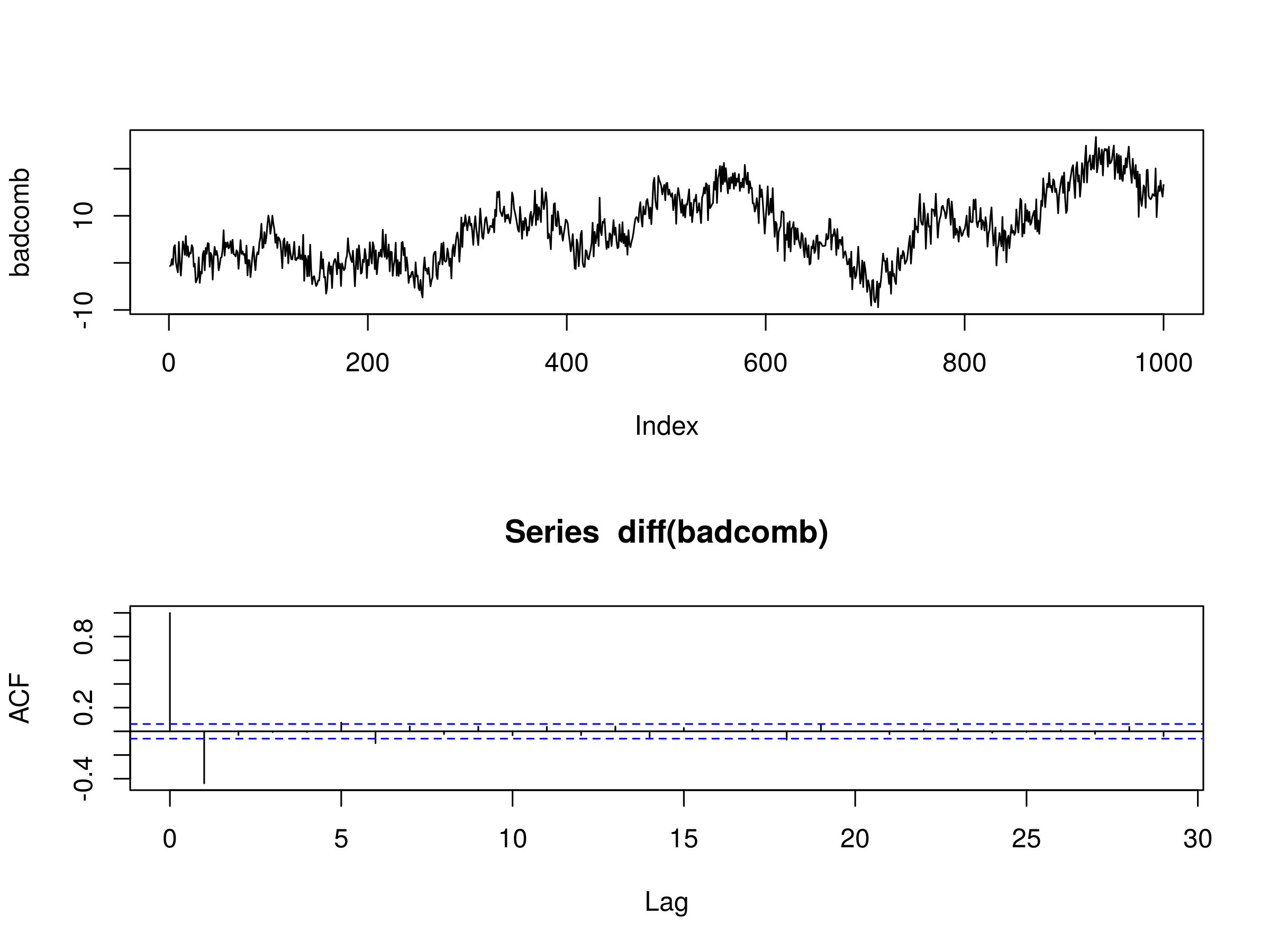 Plot of
 badcomb - the "incorrect" linear combination series - and its correlogram
In this case we do not have sufficient evidence to reject the null hypothesis of the presence of a unit root, as determined by p-value of the Augmented Dickey-Fuller test. This makes sense as we arbitrarily chose the linear combination of $a$ and $b$ rather than setting them to the correct values of $p=2$ and $b=-1$ to form a stationary series.
Next Steps
In this article we examined multiple unit root tests for assessing whether a linear combination of time series was stationary, that is, whether the two series were cointegrated.
In future articles we are going to consider full implementations of mean reverting trading strategies for daily equities and ETFs data using QSTrader based on these cointegration tests.
In addition we will extend our analysis to cointegration across more than two assets leading to trading strategies that take advantage of cointegrated portfolios.
References
- [1] Cowpertwait, P.S.P., Metcalfe, A.V. (2009) Introductory Time Series with R, Springer
- [2] Dickey, D.A., Fuller, W.A. (1979) "Distribution of the Estimators for Autoregressive Time Series with a Unit Root", Journal of the American Statistical Association 74 (366): 427-431
- [3] Pfaff, B. (2010) Analysis of Integrated and Cointegrated Time Series with R, 2nd Ed., Springer
- [4] Phillips, P.C.B., Ouliaris, S. (1990) "Asymptotic Properties of Residual Based Tests for Cointegration", Econometrica 58 (1): 165-193
- [5] Phillips, P.C.B., Perron, P. (1988) "Testing for a Unit Root in Time Series Regression", Biometrika 75 (2): 335–346
- [6] Said, S.E., Dickey, D.A. (1984) "Testing for Unit Roots in Autoregressive-Moving Average Models of Unknown Order", Biometrika 71 (3): 599-607
- [7] Zivot, E. (2006) Economics 584: Time Series Economics, Course Notes


