Updated to Python 3.8 June 2022
To date on QuantStart we have introduced Bayesian statistics, inferred a binomial proportion analytically with conjugate priors and have described the basics of Markov Chain Monte Carlo via the Metropolis algorithm. In this article we are going to introduce regression modelling in the Bayesian framework and carry out inference using the PyMC library.

We will begin by recapping the classical, or frequentist, approach to multiple linear regression. Then we will discuss how a Bayesian thinks of linear regression. We will briefly describe the concept of a Generalised Linear Model (GLM), as this is necessary to understand the clean syntax of model descriptions in PyMC.
Subsequent to the description of these models we will simulate some linear data with noise and then use PyMC to produce posterior distributions for the parameters of the model. If you recall, this is the same procedure we carried out when discussing time series models such as ARMA and GARCH. This "simulate and fit" process not only helps us understand the model, but also checks that we are fitting it correctly when we know the "true" parameter values.
Let's now turn our attention to the frequentist approach to linear regression.
Frequentist Linear Regression
The frequentist, or classical, approach to multiple linear regression assumes a model of the form (Hastie et al):
\begin{eqnarray} f \left( \mathbf{X} \right) = \beta_0 + \sum_{j=1}^p \mathbf{X}_j \beta_j + \epsilon = \beta^T \mathbf{X} + \epsilon \end{eqnarray}Where, $\beta^T$ is the transpose of the coefficient vector $\beta$ and $\epsilon \sim \mathcal{N}(0,\sigma^2)$ is the measurement error, normally distributed with mean zero and standard deviation $\sigma$.
That is, our model $f(\mathbf{X})$ is linear in the predictors, $\mathbf{X}$, with some associated measurement error.
If we have a set of training data $(x_1, y_1), \ldots, (x_N, y_N)$ then the goal is to estimate the $\beta$ coefficients, which provide the best linear fit to the data. Geometrically, this means we need to find the orientation of the hyperplane that best linearly characterises the data.
"Best" in this case means minimising some form of error function. The most popular method to do this is via ordinary least squares (OLS). If we define the residual sum of squares (RSS), which is the sum of the squared differences between the outputs and the linear regression estimates:
\begin{eqnarray} \text{RSS}(\beta) &=& \sum_{i=1}^{N} (y_i - f(x_i))^2 \\ &=& \sum_{i=1}^{N} (y_i - \beta^T x_i)^2 \end{eqnarray}Then the goal of OLS is to minimise the RSS, via adjustment of the $\beta$ coefficients. Although we won't derive it here (see Hastie et al for details) the Maximum Likelihood Estimate of $\beta$, which minimises the RSS, is given by:
\begin{eqnarray} \hat{\beta} = (\mathbf{X}^T \mathbf{X})^{-1} \mathbf{X}^T \mathbf{y} \end{eqnarray}To make a subsequent prediction $y_{N+1}$, given some new data $x_{N+1}$, we simply multiply the components of $x_{N+1}$ by the associated $\beta$ coefficients and obtain $y_{N+1}$.
The important point here is that $\hat{\beta}$ is a point estimate. This means that it is a single value in $\mathbb{R}^{p+1}$. In the Bayesian formulation we will see that the interpretation differs substantially.
Bayesian Linear Regression
In a Bayesian framework, linear regression is stated in a probabilistic manner. That is, we reformulate the above linear regression model to use probability distributions. The syntax for a linear regression in a Bayesian framework looks like this:
\begin{eqnarray} \mathbf{y} \sim \mathcal{N} \left(\beta^T \mathbf{X}, \sigma^2 \mathbf{I} \right) \end{eqnarray}In words, our response datapoints $\mathbf{y}$ are sampled from a multivariate normal distribution that has a mean equal to the product of the $\beta$ coefficients and the predictors, $\mathbf{X}$, and a variance of $\sigma^2$. Here, $\mathbf{I}$ refers to the identity matrix, which is necessary because the distribution is multivariate.
This is a very different formulation to the frequentist approach. In the frequentist setting there is no mention of probability distributions for anything other than the measurement error. In the Bayesian formulation the entire problem is recast such that the $y_i$ values are samples from a normal distribution.
A common question at this stage is "What is the benefit of doing this?". What do we get out of this reformulation? There are two main reasons for doing so (Wiecki):
- Prior Distributions: If we have any prior knowledge about the parameters $\beta$, then we can choose prior distributions that reflect this. If we don't, then we can still choose non-informative priors.
- Posterior Distributions: As mentioned above, the frequentist MLE value for our regression coefficients, $\hat{\beta}$, was only a single point estimate. In the Bayesian formulation we receive an entire probability distribution that characterises our uncertainty on the different $\beta$ coefficients. The immediate benefit of this is that after taking into account any data we can quantify our uncertainty in the $\beta$ parameters via the variance of this posterior distribution. A larger variance indicates more uncertainty.
While the above formula for the Bayesian approach may appear succinct, it doesn't really give us much clue as to how to specify a model and sample from it using Markov Chain Monte Carlo. In the next few sections we will use PyMC to formulate and utilise a Bayesian linear regression model.
Bayesian Linear Regression with PyMC
In this section we are going to carry out a time-honoured approach to statistical examples, namely to simulate some data with properties that we know, and then fit a model to recover these original properties. I have used this technique many times in the past, principally in the articles on time series analysis.
While it may seem contrived to go through such a procedure, there are in fact two major benefits. The first is that it helps us understand exactly how to fit the model. In order to do so, we have to understand it first. Thus it helps us gain intuition into how the model works. The second reason is that it allows us to see how the model performs (i.e. the values and uncertainty it returns) in a situation where we actually know the true values trying to be estimated.
Our approach will make use of numpy and pandas to simulate the data, use seaborn to plot it, and ultimately use the Generalised Linear Models (GLM) module of PyMC to formulate a Bayesian linear regression and sample from it, on our simulated data set.
The following analysis is based mainly on a collection of blog posts written by Thomas Wiecki and Jonathan Sedar, along with more theoretical Bayesian underpinnings from Gelman et al.
What are Generalised Linear Models?
Before we begin discussing Bayesian linear regression, I want to briefly outline the concept of a Generalised Linear Model (GLM), as we'll be using these to formulate our model in PyMC.
A Generalised Linear Model is a flexible mechanism for extending ordinary linear regression to more general forms of regression, including logistic regression (classification) and Poisson regression (used for count data), as well as linear regression itself.
GLMs allow for response variables that have error distributions other than the normal distribution (see $\epsilon$ above, in the frequentist section). The linear model is related to the response/outcome, $\mathbf{y}$, via a "link function", and is assumed to be generated from a statistical distribution from the exponential distribution family. This family of distributions encompasses many common distributions including the normal, gamma, beta, chi-squared, Bernoulli, Poisson and others.
The mean of this distribution, $\mathbf{\mu}$ depends on $\mathbf{X}$ via the following relation:
\begin{eqnarray} \mathbb{E}(\mathbf{y}) = \mu = g^{-1}(\mathbf{X}\beta) \end{eqnarray}Where $g$ is the link function. The variance is often some function, $V$, of the mean:
\begin{eqnarray} \text{Var}(\mathbf{y}) = V(\mathbb{E}(\mathbf{y})) = V(g^{-1}(\mathbf{X}\beta)) \end{eqnarray}In the frequentist setting, as with ordinary linear regression above, the unknown $\beta$ coefficients are estimated via a maximum likelihood approach.
We're not going to discuss GLMs in depth here as they are not the focus of the article. We are interested in them because we will be using the glm module from PyMC, which was written by Thomas Wiecki and others, in order to easily specify our Bayesian linear regression.
Simulating Data and Fitting the Model with PyMC
Before we utilise PyMC to specify and sample a Bayesian model, we need to simulate some noisy linear data. The following snippet carries this out (this is modified and extended from Jonathan Sedar's post). First we create our x values, which are equally spaced floating point values between 0 and 1. To do this we can use np.linspace(). Then we use a linear model to simulate our y values with an intercept of 1 and a slope of 2. To create our noisy dataset we add a value, epsilon, to the values of y. These values are generated using numpy's RandomState.normal(), which draws random samples from a normal distribution. We set the mean or "loc" to be equal to 0 and the standard deviation or "scale" to be equal to 0.5. We also fix the random seed to ensure that we always draw the same set of numbers when we run the code.
import matplotlib.pyplot as plt
import numpy as np
import pandas as pd
import seaborn as sns


sns.set(style="darkgrid", palette="muted")


def simulate_linear_data(
    start, stop, N, beta_0, beta_1, eps_mean, eps_sigma_sq
):
    """
    Simulate a random dataset using a noisy
    linear process.

    Parameters
    ----------
    N: `int`
        Number of data points to simulate
    beta_0: `float`
        Intercept
    beta_1: `float`
        Slope of univariate predictor, X

    Returns
    -------
    df: `pd.DataFrame`
        A DataFrame containing the x and y values.
    """
    # Create a pandas DataFrame with column 'x' containing
    # N uniformly sampled values between 0.0 and 1.0
    df = pd.DataFrame(
        {"x":
            np.linspace(start, stop, num=N)
        }
    )
    # Use a linear model (y ~ beta_0 + beta_1*x + epsilon) to
    # generate a column 'y' of responses based on 'x'
    df["y"] = beta_0 + beta_1*df["x"] + np.random.RandomState(s).normal(
        eps_mean, eps_sigma_sq, N
    )
    return df


def plot_simulated_data(df):
    """
    Plot the simulated data with sns.lmplot()

    Parameters
    ----------
    df: `pd.DataFrame`
        A DataFrame containing the x and y values.
    """
    # Plot the data, and a frequentist linear regression fit
    # using the seaborn package
    sns.lmplot(x="x", y="y", data=df, height=10)
    plt.xlim(0.0, 1.0)
    plt.show()


if __name__ == "__main__":
    # These are our "true" parameters
    beta_0 = 1.0  # Intercept
    beta_1 = 2.0  # Slope

    # Simulate 100 data points between 0 and 1, with a variance of 0.5
    start = 0
    stop = 1
    N = 100
    eps_mean = 0.0
    eps_sigma_sq = 0.5

    # Fix Random Seed
    s = 42

    # Simulate the "linear" data using the above parameters
    df = simulate_linear_data(
        start, stop, N, beta_0, beta_1, eps_mean, eps_sigma_sq
    )
    # Plot the simulated data
    plot_simulated_data(df)
The output is given in the following figure:
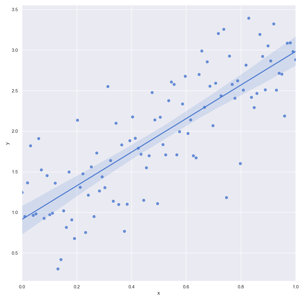
We've simulated 100 datapoints, with an intercept $\beta_0=1$ and a slope of $\beta_1=2$. The epsilon values are normally distributed with a mean of zero and variance $\sigma^2=\frac{1}{2}$. The data has been plotted using the sns.lmplot method. In addition, the method uses a frequentist MLE approach to fit a linear regression line to the data.
Now that we have carried out the simulation we want to fit a Bayesian linear regression to the data. This is where PyMC's glm module comes in. In conjunction with the Bambi library as described in the PyMC tutorial, it uses a model specification syntax that is similar to how R specifies models. The bambi library takes a formula linear model specifier from which it creates a design matrix. bambi then adds random variables for each of the coefficients and an appopriate likelihood to the model. If bambi is not installed, you can install it with pip install bambi.
Finally, we are going to use the No-U-Turn Sampler(NUTS) to carry out the actual inference and then plot the trace of the model. We will draw 5000 samples from the posterior distribution and use the first 500 samples to tune the model then discard them as "burn in". PyMC allows you to sample multiple chains based on the number of CPUs in your system. By default it is set to the number of cores in the system, here we have explicitly set it to one.
# NEW
import bambi as bmb
import matplotlib.pyplot as plt
import numpy as np
import pandas as pd
# NEW
import pymc as pm
import seaborn as sns

...


def glm_mcmc_inference(df, iterations=5000):
    """
    Calculates the Markov Chain Monte Carlo trace of
    a Generalised Linear Model Bayesian linear regression
    model on supplied data.

    Parameters
    ----------
    df: `pd.DataFrame`
        DataFrame containing the data
    iterations: `int`
        Number of iterations to carry out MCMC for
    """
    # Create the glm using the Bambi model syntax
    model = bmb.Model("y ~ x", df)

    # Fit the model using a NUTS (No-U-Turn Sampler)
    trace = model.fit(
        draws=5000,
        tune=500,
        discard_tuned_samples=True,
        chains=1,
        progressbar=True)
    return trace


def plot_glm_model(trace):
    """
    Plot the trace generated from fitting the model.

    Parameters
    ----------
    trace: `tracepymc.backends.base.MultiTrace`
        A MultiTrace or ArviZ InferenceData object that contains the samples.
    """
    pm.plot_trace(trace)
    plt.tight_layout()
    plt.show()


if __name__ == "__main__":
    # These are our "true" parameters
    beta_0 = 1.0  # Intercept
    beta_1 = 2.0  # Slope

    # Simulate 100 data points between 0 and 1, with a variance of 0.5
    start = 0
    stop = 1
    N = 100
    eps_mean = 0.0
    eps_sigma_sq = 0.5

    # Fix Random Seed
    s = 42

    # Simulate the "linear" data using the above parameters
    df = simulate_linear_data(
        start, stop, N, beta_0, beta_1, eps_mean, eps_sigma_sq
    )
    # Plot the simulated data
    plot_simulated_data(df)

    # NEW
    # Fit the GLM
    trace = glm_mcmc_inference(df, iterations=5000)
    # Plot the GLM
    plot_glm_model(trace))
The output of the script is as follows:
Auto-assigning NUTS sampler...
Initializing NUTS using jitter+adapt_diag...
Multiprocess sampling (2 chains in 2 jobs)
NUTS: [Intercept, x, y_sigma]
[-----------------]Sampling 1 chains for 500 tune and 5_000 draw iterations (500 + 5_000 draws total) took 12 seconds.
The traceplot is given in the following figure:
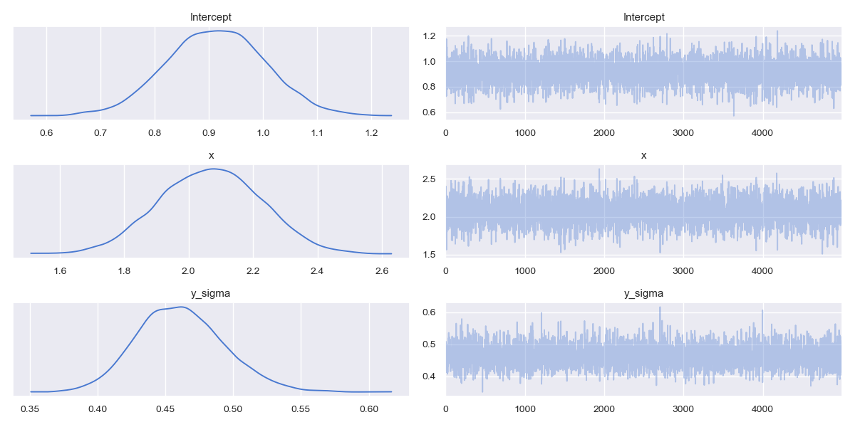
We covered the basics of traceplots in the previous article on the Metropolis MCMC algorithm. Recall that Bayesian models provide a full posterior probability distribution for each of the model parameters, as opposed to a frequentist point estimate.
On the left side of the panel we can see marginal distributions for each parameter of interest. Notice that the intercept $\beta_0$ distribution has its mode/maximum posterior estimate almost at 1, close to the true parameter of $\beta_0=1$. The estimate for the slope (x) $\beta_1$ parameter has a mode at approximately 2.1, close to the true parameter value of $\beta_1=2$. The y_sigma error parameter associated with the model measurement noise has a mode of approximately 0.46, which is a little off compared to the true value of $\epsilon=0.5$.
In all cases there is a reasonable variance associated with each marginal posterior, telling us that there is some degree of uncertainty in each of the values. Were we to simulate more data, and carry out more samples, this variance would likely decrease.
The key point here is that we do not receive a single point estimate for a regression line, i.e. "a line of best fit", as in the frequentist case. Instead we receive a distribution of likely regression lines.
We can plot these lines along with the true regression line and the simulated data we created earlier. We begin by creating our figure where our x axis is a linearly spaced floating point number between 0 and 1 with 100 steps. We then plot our simulated data using Matplotlib's plt.scatter and our original DataFrame, df.
We can access the numeric data for the posterior distributions from within the trace object created by the model. The trace inference data has the following groups; posterior, log_likelihood, sample_stats, observed_data. The posterior group contains the values of the 5000 draws from the posterior distributon of the intercept and slope (x). These arrays are of shape(1, 5000). The first value represents the number of chains, the second is the number of draws. This dataset also features a method to_numpy() which converts the data to a numpy array. So in order to get the values for the intercepts into an array that we can sample from and plot we need to use the following code: trace.posterior.Intercept.to_numpy()[0]. To get our slope data we do the same but replace Intercepts with x trace.posterior.x.to_numpy()[0]. We now have two arrays with the numeric values from the posterior distributions for our slopes and intercepts.
In order to plot a sample of 100 lines we need to pick 100 of these values from our arrays. First we create a sample index list by creating a list of random integers using numpy's random.randint() method. Then we loop through the array with our index value and create a line using the intercept and slope, plotting the line on our graph. Finally we plot our true regression line using the beta_0 and beta_1 variables from our simulated data. The code snippet below produces such a plot:
..
def plot_regression_lines(trace, df, N):
    """
    Plot the simulated data with true and estimated regression lines.

    Parameters
    ----------
    trace: `tracepymc.backends.base.MultiTrace`
        A MultiTrace or ArviZ InferenceData object that contains the samples.
    df: `pd.DataFrame`
        DataFrame containing the data
    N: `int`
        Number of data points to simulate
    """
    fig, ax = plt.subplots(figsize=(7, 7))
    # define x axis ticks
    x = np.linspace(0, 1, N)
    # plot simulated data observations
    ax.scatter(df['x'], df['y'])
    # extract slope and intercept draws from PyMC trace
    intercepts = trace.posterior.Intercept.to_numpy()[0]
    slopes = trace.posterior.x.to_numpy()[0]
    # plot 100 random samples from the slope and intercept draws
    sample_indexes = np.random.randint(len(intercepts), size=100)
    for i in sample_indexes:
        y_line = intercepts[i] + slopes[i] * x
        ax.plot(x, y_line, c='black', alpha=0.07)
    # plot true regression line
    y = beta_0 + beta_1*x
    ax.plot(x, y, label="True Regression Line", lw=3., c="green")
    ax.legend(loc=0)
    ax.set_xlim(0.0, 1.0)
    ax.set_ylim(0.0, 4.0)
    plt.show()


if __name__ == "__main__":
    # These are our "true" parameters
    beta_0 = 1.0  # Intercept
    beta_1 = 2.0  # Slope

    # Simulate 100 data points between 0 and 1, with a variance of 0.5
    start = 0
    stop = 1
    N = 100
    eps_mean = 0.0
    eps_sigma_sq = 0.5

    # Fix Random Seed
    s = 42

    # Simulate the "linear" data using the above parameters
    df = simulate_linear_data(
        start, stop, N, beta_0, beta_1, eps_mean, eps_sigma_sq
    )
    # Plot the simulated data
    plot_simulated_data(df)

    # Fit the GLM
    trace = glm_mcmc_inference(df, iterations=5000)
    # Plot the GLM
    plot_glm_model(trace)
    # NEW
    plot_regression_lines(trace, df, N)
We can see the sampled range of posterior regression lines in the following figure:
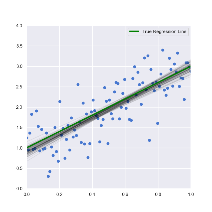
The main takeaway here is that there is uncertainty in the location of the regression line as sampled by the Bayesian model. However, it can be seen that the range is relatively narrow and that the set of samples is not too dissimilar to the "true" regression line itself.
Next Steps
In the previous article we looked at a basic MCMC method called the Metropolis algorithm. We mentioned in that article that we wanted to see how various "flavours" of MCMC work "under the hood". In future articles we will consider the Gibbs Sampler, Hamiltonian Sampler and No-U-Turn Sampler, all of which are utilised in the main Bayesian software packages.
We will eventually discuss robust regression and hierarchical linear models, a powerful modelling technique made tractable by rapid MCMC implementations. From a quantitative finance point of view we will also take a look at a stochastic volatility model using PyMC and see how we can use this model to form trading algorithms.
Bibliographic Note
An introduction to frequentist linear regression can be found in James et al (2013). A more technical overview, including subset selection methods, can be found in Hastie et al (2009). Gelman et al (2013) discuss Bayesian linear models in depth at a reasonably technical level.
This article is heavily influenced by previous blog posts by Thomas Wiecki including his discussion of Bayesian GLMs here, as well as Jonathan Sedar's posts.
References
- Gelman, A. et al (2013) Bayesian Data Analysis, 3rd Edition, Chapman and Hall/CRC
- Hastie, T., Tibshirani, R., Friedman, J. (2009) The Elements of Statistical Learning, Springer
- Hoffman, M.D., and Gelman, A. (2011) "The No-U-Turn Sampler: Adaptively Setting Path Lengths in Hamiltonian Monte Carlo, arXiv:1111.4246 [stat.CO]
- James, G., Witten, D., Hastie, T., Tibshirani, R. (2013) An Introduction to Statistical Learning, Springer
- Sedar, J. (2016) Bayesian Inference with PyMC3 - Part 1
- Wiecki, T. (2015) The Inference Button: Bayesian GLMs made easy with PyMC3, https://twiecki.github.io/blog/2013/08/12/bayesian-glms-1/
Full Code
import bambi as bmb
import matplotlib.pyplot as plt
import numpy as np
import pandas as pd
import pymc as pm
import seaborn as sns


sns.set(style="darkgrid", palette="muted")


def simulate_linear_data(
    start, stop, N, beta_0, beta_1, eps_mean, eps_sigma_sq
):
    """
    Simulate a random dataset using a noisy
    linear process.

    Parameters
    ----------
    N: `int`
        Number of data points to simulate
    beta_0: `float`
        Intercept
    beta_1: `float`
        Slope of univariate predictor, X

    Returns
    -------
    df: `pd.DataFrame`
        A DataFrame containing the x and y values
    """
    # Create a pandas DataFrame with column 'x' containing
    # N uniformly sampled values between 0.0 and 1.0
    df = pd.DataFrame(
        {"x":
            np.linspace(start, stop, num=N)
        }
    )
    # Use a linear model (y ~ beta_0 + beta_1*x + epsilon) to
    # generate a column 'y' of responses based on 'x'
    df["y"] = beta_0 + beta_1*df["x"] + np.random.RandomState(s).normal(
        eps_mean, eps_sigma_sq, N
    )
    return df


def plot_simulated_data(df):
    """
    Plot the simulated data with sns.lmplot().

    Parameters
    ----------
    df: `pd.DataFrame`
        A DataFrame containing the x and y values
    """
    # Plot the data, and a frequentist linear regression fit
    # using the seaborn package
    sns.lmplot(x="x", y="y", data=df, height=10)
    plt.xlim(0.0, 1.0)
    plt.show()


def glm_mcmc_inference(df, iterations=5000):
    """
    Calculates the Markov Chain Monte Carlo trace of
    a Generalised Linear Model Bayesian linear regression
    model on supplied data.

    Parameters
    ----------
    df: `pd.DataFrame`
        DataFrame containing the data
    iterations: `int`
        Number of iterations to carry out MCMC for
    """
    # Create the glm using the Bambi model syntax
    model = bmb.Model("y ~ x", df)

    # Fit the model using a NUTS (No-U-Turn Sampler)
    trace = model.fit(
        draws=5000,
        tune=500,
        discard_tuned_samples=True,
        chains=1,
        progressbar=True)
    return trace


def plot_glm_model(trace):
    """
    Plot the trace generated from fitting the model.

    Parameters
    ----------
    trace: `tracepymc.backends.base.MultiTrace`
        A MultiTrace or ArviZ InferenceData object that contains the samples.
    """
    pm.plot_trace(trace)
    plt.tight_layout()
    plt.show()


def plot_regression_lines(trace, df, N):
    """
    Plot the simulated data with True and estimated regression lines.

    Parameters
    ----------
    trace: `tracepymc.backends.base.MultiTrace`
        A MultiTrace or ArviZ InferenceData object that contains the samples.
    df: `pd.DataFrame`
        DataFrame containing the data
    N: `int`
        Number of data points to simulate
    """
    fig, ax = plt.subplots(figsize=(7, 7))
    # define x axis ticks
    x = np.linspace(0, 1, N)
    # plot simulated data observations
    ax.scatter(df['x'], df['y'])
    # extract slope and intercept draws from PyMC trace
    intercepts = trace.posterior.Intercept.to_numpy()[0]
    slopes = trace.posterior.x.to_numpy()[0]
    # plot 100 random samples from the slope and intercept draws
    sample_indexes = np.random.randint(len(intercepts), size=100)
    for i in sample_indexes:
        y_line = intercepts[i] + slopes[i] * x
        ax.plot(x, y_line, c='black', alpha=0.07)
    # plot true regression line
    y = beta_0 + beta_1*x
    ax.plot(x, y, label="True Regression Line", lw=3., c="green")
    ax.legend(loc=0)
    ax.set_xlim(0.0, 1.0)
    ax.set_ylim(0.0, 4.0)
    plt.show()


if __name__ == "__main__":
    # These are our "true" parameters
    beta_0 = 1.0  # Intercept
    beta_1 = 2.0  # Slope

    # Simulate 100 data points between 0 and 1, with a variance of 0.5
    start = 0
    stop = 1
    N = 100
    eps_mean = 0.0
    eps_sigma_sq = 0.5

    # Fix Random Seed
    s = 42

    # Simulate the "linear" data using the above parameters
    df = simulate_linear_data(
        start, stop, N, beta_0, beta_1, eps_mean, eps_sigma_sq
    )
    # Plot the simulated data
    plot_simulated_data(df)

    # Fit the GLM
    trace = glm_mcmc_inference(df, iterations=5000)
    # Plot the GLM
    plot_glm_model(trace)
    plot_regression_lines(trace, df, N)


