In the previous set of articles (Parts 1, 2 and 3) we went into significant detail about the AR(p), MA(q) and ARMA(p,q) linear time series models. We used these models to generate simulated data sets, fitted models to recover parameters and then applied these models to financial equities data.

In this article we are going to discuss an extension of the ARMA model, namely the Autoregressive Integrated Moving Average model, or ARIMA(p,d,q) model. We will see that it is necessary to consider the ARIMA model when we have non-stationary series. Such series occur in the presence of stochastic trends.

Quick Recap and Next Steps

To date we have considered the following models (the links will take you to the appropriate articles):

• Discrete White Noise
• Random Walk
• Autoregressive Model of order p, AR(p)
• Moving Average Model of order q, MA(q)
• Autoregressive Moving Average Model of order p,q, ARMA(p,q)

We have steadily built up our understanding of time series with concepts such as serial correlation, stationarity, linearity, residuals, correlograms, simulating, fitting, seasonality, conditional heteroscedasticity and hypothesis testing.

As of yet we have not carried out any prediction or forecasting from our models and so have not had any mechanism for producing a trading system or equity curve.

Once we have studied ARIMA (in this article), ARCH and GARCH (in the next articles), we will be in a position to build a basic long-term trading strategy based on prediction of stock market index returns.

Despite the fact that I have gone into a lot of detail about models which we know will ultimately not have great performance (AR, MA, ARMA), we are now well-versed in the process of time series modeling.

This means that when we come to study more recent models (and even those currently in the research literature), we will have a significant knowledge base on which to draw, in order to effectively evaluate these models, instead of treating them as a "turn key" prescription or "black box".

More importantly, it will provide us with the confidence to extend and modify them on our own and understand what we are doing when we do it!

I'd like to thank you for being patient so far, as it might seem that these articles are far away from the "real action" of actual trading. However, true quantitative trading research is careful, measured and takes significant time to get right. There is no quick fix or "get rich scheme" in quant trading.

We're very nearly ready to consider our first trading model, which will be a mixture of ARIMA and GARCH, so it is imperative that we spend some time understanding the ARIMA model well!

Once we have built our first trading model, we are going to consider more advanced models such as long-memory processes, state-space models (i.e. the Kalman Filter) and Vector Autoregressive (VAR) models, which will lead us to other, more sophisticated, trading strategies.

Autoregressive Integrated Moving Average (ARIMA) Models of order p, d, q

Rationale

ARIMA models are used because they can reduce a non-stationary series to a stationary series using a sequence of differencing steps.

We can recall from the article on white noise and random walks that if we apply the difference operator to a random walk series $\{x_t \}$ (a non-stationary series) we are left with white noise $\{w_t \}$ (a stationary series):

ARIMA essentially performs this function, but does so repeatedly, $d$ times, in order to reduce a non-stationary series to a stationary one.

In order to handle other forms of non-stationarity beyond stochastic trends additional models can be used.

Seasonality effects (such as those that occur in commodity prices) can be tackled with the Seasonal ARIMA model (SARIMA), however we won't be discussing SARIMA much in this series.

Conditional heteroscedastic effects (as with volatility clustering in equities indexes) can be tackled with ARCH/GARCH.

In this article we will be considering non-stationary series with stochastic trends and fit ARIMA models to these series. We will also finally produce forecasts for our financial series.

Definitions

Prior to defining ARIMA processes we need to discuss the concept of an integrated series:

Now that we have defined an integrated series we can define the ARIMA process itself:

There are some points to note about these definitions.

Since the random walk is given by $x_t = x_{t-1} + w_t$ it can be seen that $I(1)$ is another representation, since $\nabla^1 x_t = w_t$.

If we suspect a non-linear trend then we might be able to use repeated differencing (i.e. $d > 1$) to reduce a series to stationary white noise.

In R we can use the diff command with additional parameters, e.g. diff(x, d=3) to carry out repeated differences.

Simulation, Correlogram and Model Fitting

Since we have already made use of the arima.sim command to simulate an ARMA(p,q) process, the following procedure will be similar to that carried out in Part 3 of the ARMA series.

The major difference is that we will now set $d=1$, that is, we will produce a non-stationary time series with a stochastic trending component.

As before we will fit an ARIMA model to our simulated data, attempt to recover the parameters, create confidence intervals for these parameters, produce a correlogram of the residuals of the fitted model and finally carry out a Ljung-Box test to establish whether we have a good fit.

We are going to simulate an ARIMA(1,1,1) model, with the autoregressive coefficient $\alpha=0.6$ and the moving average coefficient $\beta=-0.5$. Here is the R code to simulate and plot such a series:

> set.seed(2)
> x <- arima.sim(list(order = c(1,1,1), ar = 0.6, ma=-0.5), n = 1000)
> plot(x)

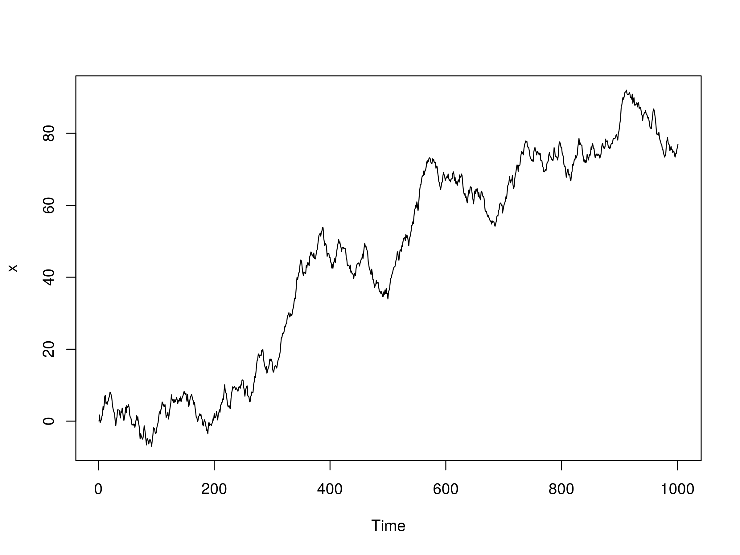Plot of simulated ARIMA(1,1,1) model with $\alpha=0.6$ and $\beta=-0.5$

Now that we have our simulated series we are going to try and fit an ARIMA(1,1,1) model to it. Since we know the order we will simply specify it in the fit:

> x.arima <- arima(x, order=c(1, 1, 1))

Call:
arima(x = x, order = c(1, 1, 1))

Coefficients:
         ar1      ma1
      0.6470  -0.5165
s.e.  0.1065   0.1189

sigma^2 estimated as 1.027:  log likelihood = -1432.09,  aic = 2870.18

The confidence intervals are calculated as:

> 0.6470 + c(-1.96, 1.96)*0.1065

0.43826 0.85574

> -0.5165 + c(-1.96, 1.96)*0.1189

-0.749544 -0.283456

Both parameter estimates fall within the confidence intervals and are close to the true parameter values of the simulated ARIMA series. Hence, we shouldn't be surprised to see the residuals looking like a realisation of discrete white noise:

> acf(resid(x.arima))

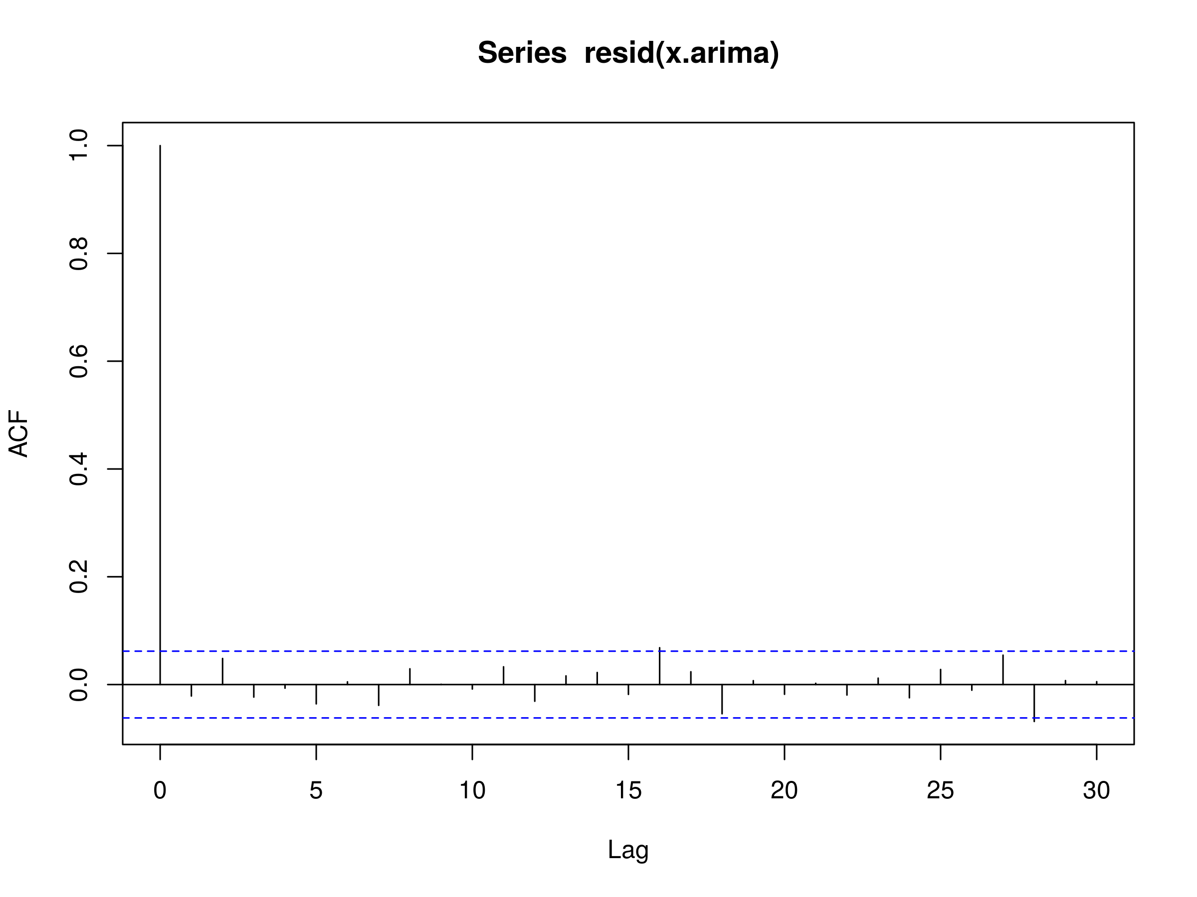Correlogram of the residuals of the fitted ARIMA(1,1,1) model

Finally, we can run a Ljung-Box test to provide statistical evidence of a good fit:

> Box.test(resid(x.arima), lag=20, type="Ljung-Box")

  Box-Ljung test

data:  resid(x.arima)
X-squared = 19.0413, df = 20, p-value = 0.5191

We can see that the p-value is significantly larger than 0.05 and as such we can state that there is strong evidence for discrete white noise being a good fit to the residuals. Hence, the ARIMA(1,1,1) model is a good fit, as expected.

Financial Data and Prediction

In this section we are going to fit ARIMA models to Amazon, Inc. (AMZN) and the S&P500 US Equity Index (^GPSC, in Yahoo Finance). We will make use of the forecast library, written by Rob J Hyndman.

Let's go ahead and install the library in R:

> install.packages("forecast")
> library(forecast)

Now we can use quantmod to download the daily price series of Amazon from the start of 2013. Since we will have already taken the first order differences of the series, the ARIMA fit carried out shortly will not require $d > 0$ for the integrated component:

> require(quantmod)
> getSymbols("AMZN", from="2013-01-01")
> amzn = diff(log(Cl(AMZN)))

As in Part 3 of the ARMA series, we are now going to loop through the combinations of $p$, $d$ and $q$, to find the optimal ARIMA(p,d,q) model. By "optimal" we mean the order combination that minimises the Akaike Information Criterion (AIC):

> azfinal.aic <- Inf
> azfinal.order <- c(0,0,0)
> for (p in 1:4) for (d in 0:1) for (q in 1:4) {
>   azcurrent.aic <- AIC(arima(amzn, order=c(p, d, q)))
>   if (azcurrent.aic < azfinal.aic) {
>     azfinal.aic <- azcurrent.aic
>     azfinal.order <- c(p, d, q)
>     azfinal.arima <- arima(amzn, order=azfinal.order)
>   }
> }

We can see that an order of $p=4$, $d=0$, $q=4$ was selected. Notably $d=0$, as we have already taken first order differences above:

> azfinal.order

4 0 4

If we plot the correlogram of the residuals we can see if we have evidence for a discrete white noise series:

> acf(resid(azfinal.arima), na.action=na.omit)

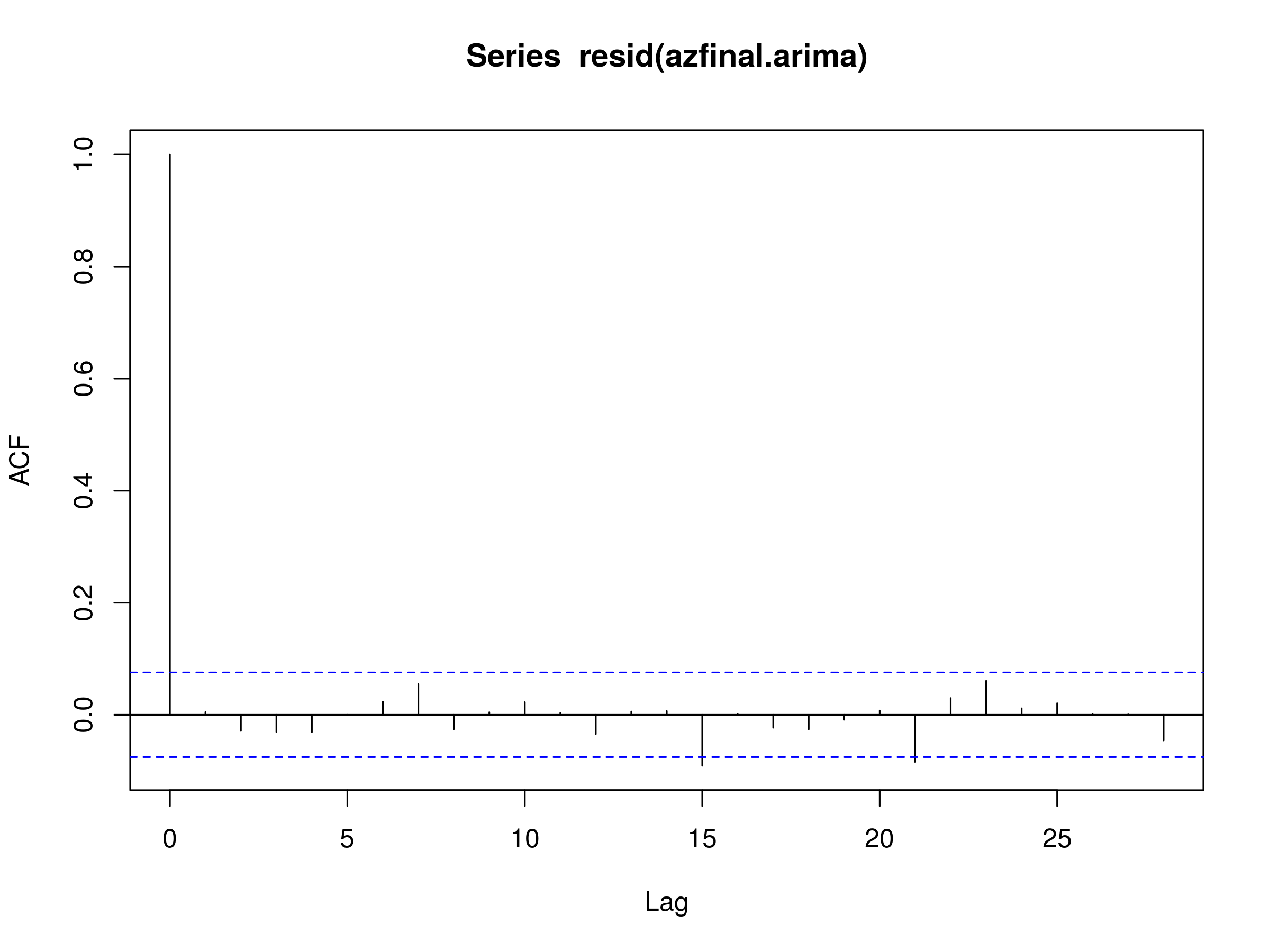Correlogram of residuals of ARIMA(4,0,4) model fitted to AMZN daily log returns

There are two significant peaks, namely at $k=15$ and $k=21$, although we should expect to see statistically significant peaks simply due to sampling variation 5% of the time. Let's perform a Ljung-Box test (see previous article) and see if we have evidence for a good fit:

> Box.test(resid(azfinal.arima), lag=20, type="Ljung-Box")

    Box-Ljung test

data:  resid(azfinal.arima)
X-squared = 12.6337, df = 20, p-value = 0.8925

As we can see the p-value is greater than 0.05 and so we have evidence for a good fit at the 95% level.

We can now use the forecast command from the forecast library in order to predict 25 days ahead for the returns series of Amazon:

> plot(forecast(azfinal.arima, h=25))

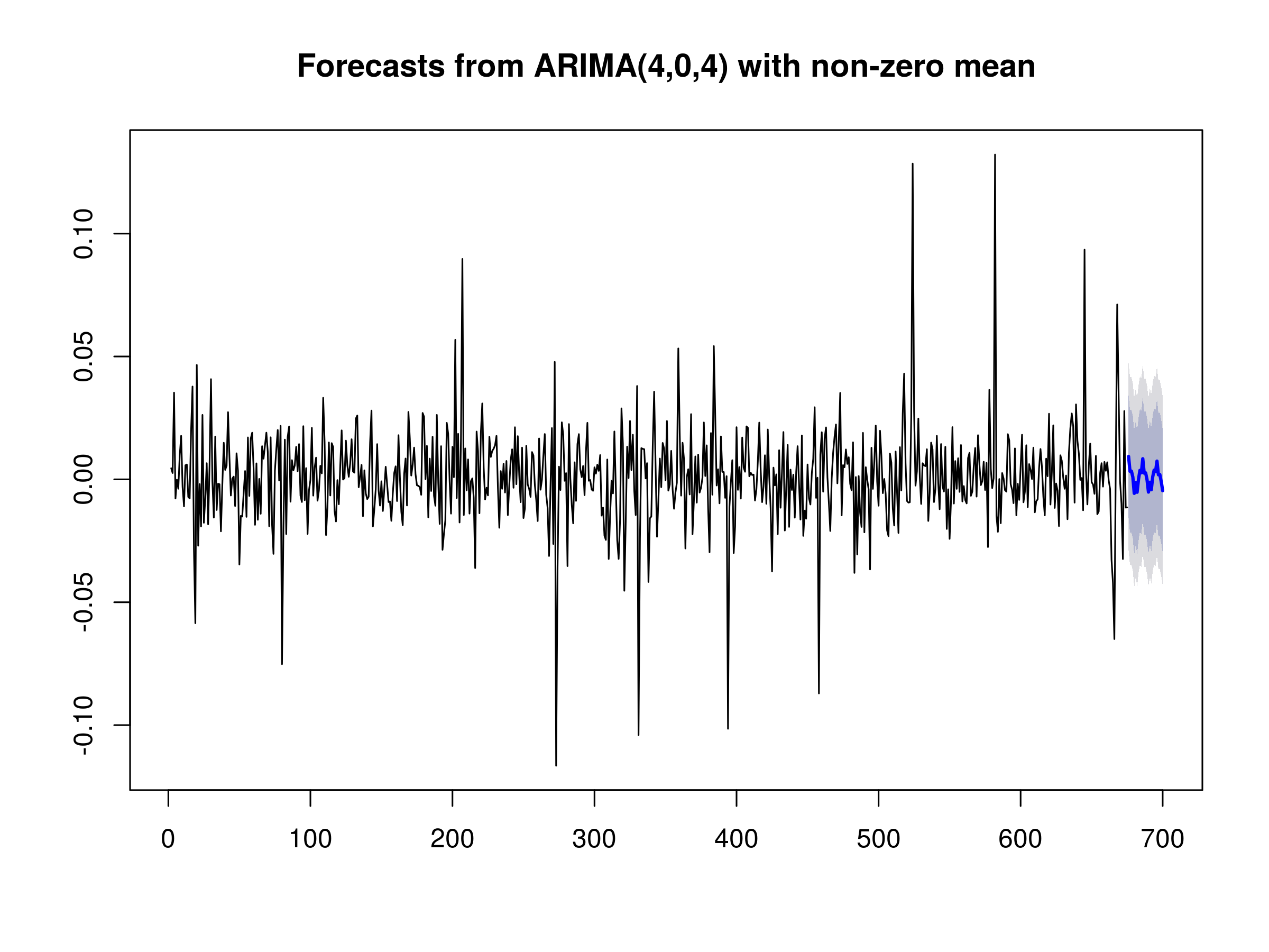25-day forecast of AMZN daily log returns

We can see the point forecasts for the next 25 days with 95% (dark blue) and 99% (light blue) error bands. We will be using these forecasts in our first time series trading strategy when we come to combine ARIMA and GARCH.

Let's carry out the same procedure for the S&P500. Firstly we obtain the data from quantmod and convert it to a daily log returns stream:

> getSymbols("^GSPC", from="2013-01-01")
> sp = diff(log(Cl(GSPC)))

We fit an ARIMA model by looping over the values of p, d and q:

> spfinal.aic <- Inf
> spfinal.order <- c(0,0,0)
> for (p in 1:4) for (d in 0:1) for (q in 1:4) {
>   spcurrent.aic <- AIC(arima(sp, order=c(p, d, q)))
>   if (spcurrent.aic < spfinal.aic) {
>     spfinal.aic <- spcurrent.aic
>     spfinal.order <- c(p, d, q)
>     spfinal.arima <- arima(sp, order=spfinal.order)
>   }
> }

The AIC tells us that the "best" model is the ARIMA(2,0,1) model. Notice once again that $d=0$, as we have already taken first order differences of the series:

> spfinal.order

2 0 1

We can plot the residuals of the fitted model to see if we have evidence of discrete white noise:

> acf(resid(spfinal.arima), na.action=na.omit)

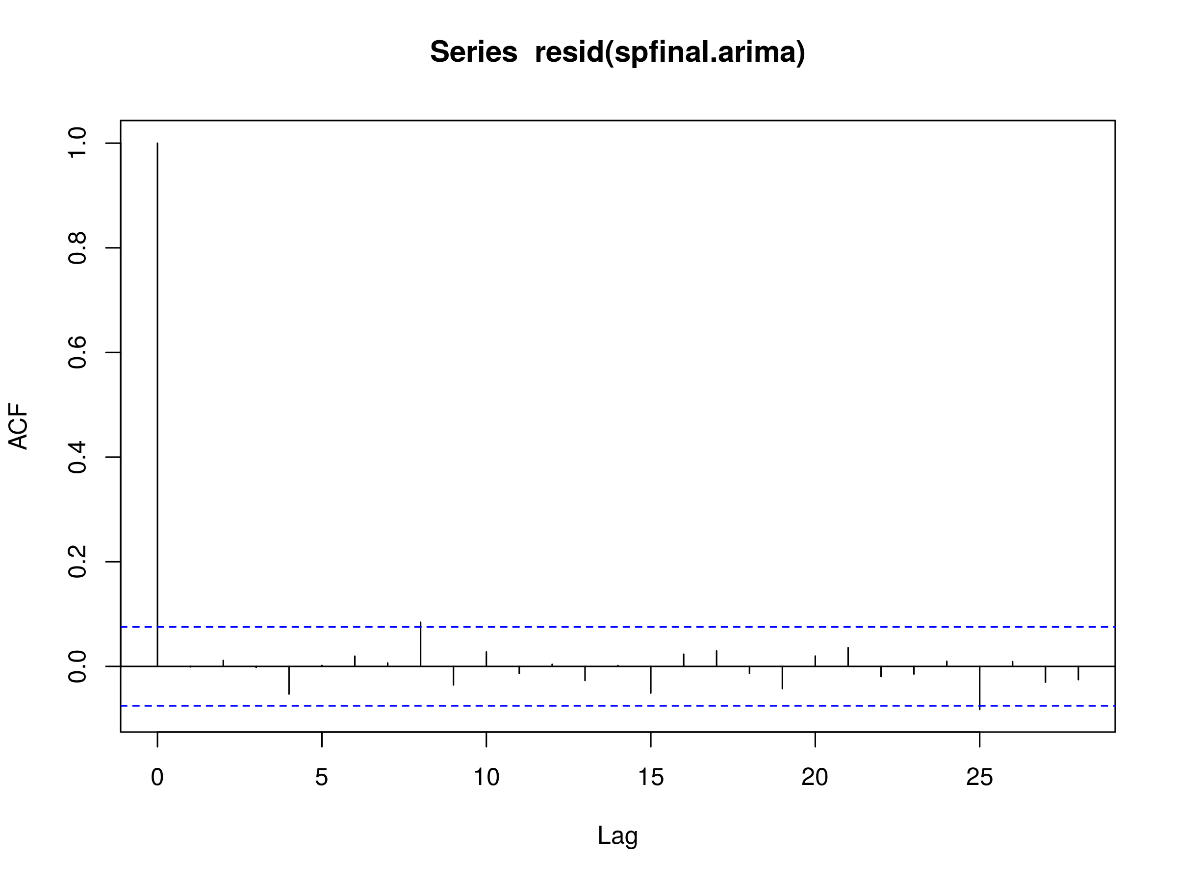Correlogram of residuals of ARIMA(2,0,1) model fitted to S&P500 daily log returns

The correlogram looks promising, so the next step is to run the Ljung-Box test and confirm that we have a good model fit:

> Box.test(resid(spfinal.arima), lag=20, type="Ljung-Box")

    Box-Ljung test

data:  resid(spfinal.arima)
X-squared = 13.6037, df = 20, p-value = 0.85

Since the p-value is greater than 0.05 we have evidence of a good model fit.

Why is it that in the previous article our Ljung-Box test for the S&P500 showed that the ARMA(3,3) was a poor fit for the daily log returns?

Notice that I deliberately truncated the S&P500 data to start from 2013 onwards in this article, which conveniently excludes the volatile periods around 2007-2008. Hence we have excluded a large portion of the S&P500 where we had excessive volatility clustering. This impacts the serial correlation of the series and hence has the effect of making the series seem "more stationary" than it has been in the past.

This is a very important point. When analysing time series we need to be extremely careful of conditionally heteroscedastic series, such as stock market indexes. In quantitative finance, trying to determine periods of differing volatility is often known as "regime detection". It is one of the harder tasks to achieve!

We'll discuss this point at length in the next article when we come to consider the ARCH and GARCH models.

Let's now plot a forecast for the next 25 days of the S&P500 daily log returns:

> plot(forecast(spfinal.arima, h=25))

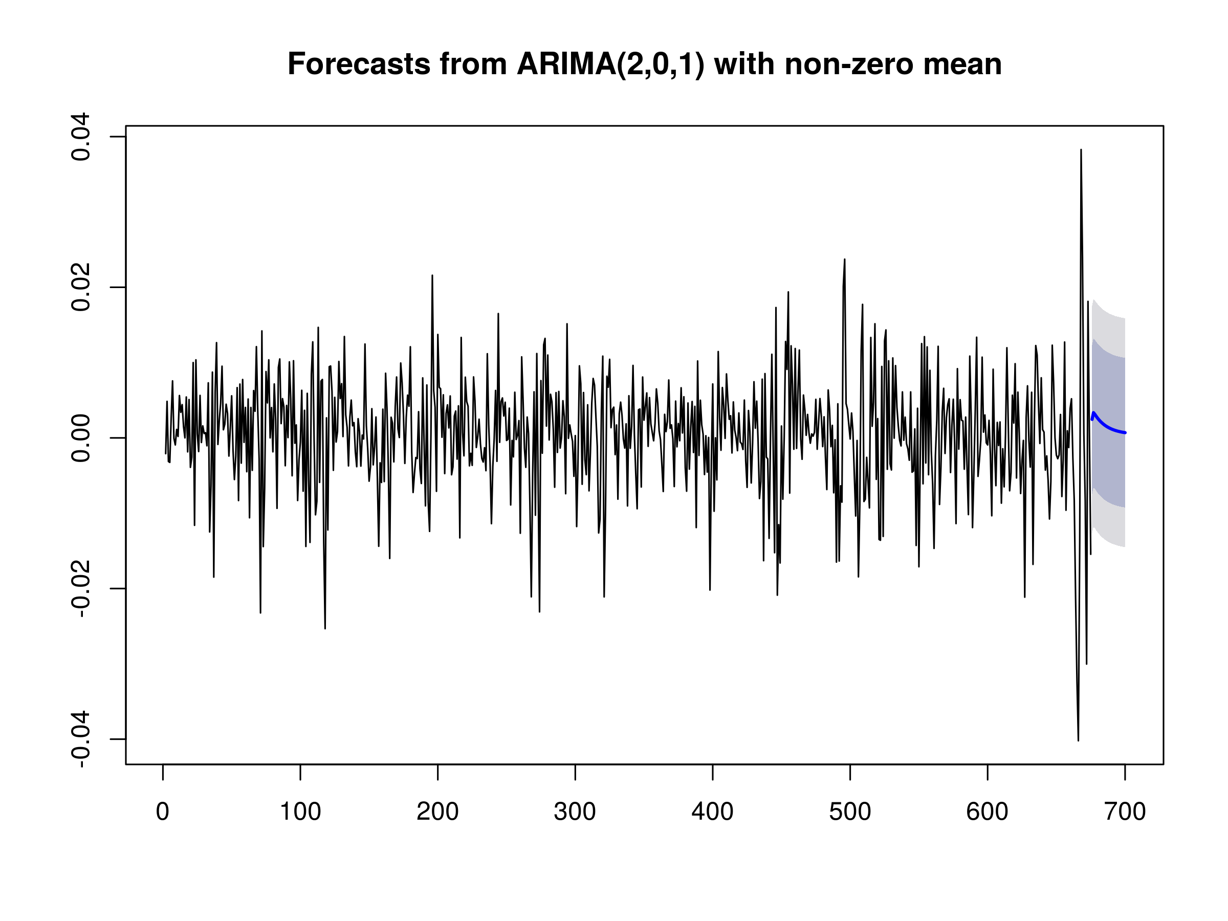25-day forecast of S&P500 daily log returns

Now that we have the ability to fit and forecast models such as ARIMA, we're very close to being able to create strategy indicators for trading.

Next Steps

In the next article we are going to take a look at the Generalised Autoregressive Conditional Heteroscedasticity (GARCH) model and use it to explain more of the serial correlation in certain equities and equity index series.

Once we have discussed GARCH we will be in a position to combine it with the ARIMA model and create signal indicators and thus a basic quantitative trading strategy.