In this article I want to show you how to apply all of the knowledge gained in the previous time series analysis posts to a trading strategy on the S&P500 US stock market index.
We will see that by combining the ARIMA and GARCH models we can significantly outperform a "Buy-and-Hold" approach over the long term.
Strategy Overview
The idea of the strategy is relatively simple but if you want to experiment with it I highly suggest reading the previous posts on time series analysis in order to understand what you would be modifying!
The strategy is carried out on a "rolling" basis:
- For each day, $n$, the previous $k$ days of the differenced logarithmic returns of a stock market index are used as a window for fitting an optimal ARIMA and GARCH model.
- The combined model is used to make a prediction for the next day returns.
- If the prediction is negative the stock is shorted at the previous close, while if it is positive it is longed.
- If the prediction is the same direction as the previous day then nothing is changed.
For this strategy I have used the maximum available data from Yahoo Finance for the S&P500. I have taken $k=500$ but this is a parameter that can be optimised in order to improve performance or reduce drawdown.
The backtest is carried out in a straightforward vectorised fashion using R. It has not been implemented in the Python event-driven backtester as of yet. Hence the performance achieved in a real trading system would likely be slightly less than you might achieve here, due to commission and slippage.
Strategy Implementation
To implement the strategy we are going to use some of the code we have previously created in the time series analysis article series as well as some new libraries including rugarch, which has been suggested to me by Ilya Kipnis over at QuantStrat Trader.
I will go through the syntax in a step-by-step fashion and then present the full implementation at the end, as well as a link to my dataset for the ARIMA+GARCH indicator. I've included the latter because it has taken me a couple of days on my dekstop PC to generate the signals!
You should be able to replicate my results in entirety as the code itself is not too complex, although it does take some time to simulate if you carry it out in full.
The first task is to install and import the necessary libraries in R:
> install.packages("quantmod")
> install.packages("lattice")
> install.packages("timeSeries")
> install.packages("rugarch")
If you already have the libraries installed you can simply import them:
> library(quantmod)
> library(lattice)
> library(timeSeries)
> library(rugarch)
With that done are going to apply the strategy to the S&P500. We can use quantmod to obtain data going back to 1950 for the index. Yahoo Finance uses the symbol "^GPSC".
We can then create the differenced logarithmic returns of the "Closing Price" of the S&P500 and strip out the initial NA value:
> getSymbols("^GSPC", from="1950-01-01")
> spReturns = diff(log(Cl(GSPC)))
> spReturns[as.character(head(index(Cl(GSPC)),1))] = 0
We need to create a vector, forecasts to store our forecast values on particular dates. We set the length foreLength to be equal to the length of trading data we have minus $k$, the window length:
> windowLength = 500
> foreLength = length(spReturns) - windowLength
> forecasts <- vector(mode="character", length=foreLength)
At this stage we need to loop through every day in the trading data and fit an appropriate ARIMA and GARCH model to the rolling window of length $k$. Given that we try 24 separate ARIMA fits and fit a GARCH model, for each day, the indicator can take a long time to generate.
We use the index d as a looping variable and loop from $k$ to the length of the trading data:
> for (d in 0:foreLength) {
We then create the rolling window by taking the S&P500 returns and selecting the values between $1+d$ and $k+d$, where $k=500$ for this strategy:
> spReturnsOffset = spReturns[(1+d):(windowLength+d)]
We use the same procedure as in the ARIMA article to search through all ARMA models with $p \in \{0 ,\ldots,5 \}$ and $q \in \{0,\ldots,5 \}$, with the exception of $p,q=0$.
We wrap the arimaFit call in an R tryCatch exception handling block to ensure that if we don't get a fit for a particular value of $p$ and $q$, we ignore it and move on to the next combination of $p$ and $q$.
Note that we set the "integrated" value of $d=0$ (this is a different $d$ to our indexing parameter!) and as such we are really fitting an ARMA model, rather than an ARIMA.
The looping procedure will provide us with the "best" fitting ARMA model, in terms of the Akaike Information Criterion, which we can then use to feed in to our GARCH model:
>     final.aic <- Inf
>     final.order <- c(0,0,0)
>     for (p in 0:5) for (q in 0:5) {
>         if ( p == 0 && q == 0) {
>             next
>         }
>
>         arimaFit = tryCatch( arima(spReturnsOffset, order=c(p, 0, q)),
>                              error=function( err ) FALSE,
>                              warning=function( err ) FALSE )
>
>         if( !is.logical( arimaFit ) ) {
>             current.aic <- AIC(arimaFit)
>             if (current.aic < final.aic) {
>                 final.aic <- current.aic
>                 final.order <- c(p, 0, q)
>                 final.arima <- arima(spReturnsOffset, order=final.order)
>             }
>         } else {
>             next
>         }
>     }
In the next code block we are going to use the rugarch library, with the GARCH(1,1) model. The syntax for this requires us to set up a ugarchspec specification object that takes a model for the variance and the mean. The variance receives the GARCH(1,1) model while the mean takes an ARMA(p,q) model, where $p$ and $q$ are chosen above. We also choose the sged distribution for the errors.
Once we have chosen the specification we carry out the actual fitting of ARMA+GARCH using the ugarchfit command, which takes the specification object, the $k$ returns of the S&P500 and a numerical optimisation solver. We have chosen to use hybrid, which tries different solvers in order to increase the likelihood of convergence:
>     spec = ugarchspec(
>                 variance.model=list(garchOrder=c(1,1)),
>                 mean.model=list(armaOrder=c(final.order[1], final.order[3]), include.mean=T),
>                 distribution.model="sged")
>
>     fit = tryCatch(
>       ugarchfit(
>         spec, spReturnsOffset, solver = 'hybrid'
>       ), error=function(e) e, warning=function(w) w
>     )
If the GARCH model does not converge then we simply set the day to produce a "long" prediction, which is clearly a guess. However, if the model does converge then we output the date and tomorrow's prediction direction (+1 or -1) as a string at which point the loop is closed off.
In order to prepare the output for the CSV file I have created a string that contains the data separated by a comma with the forecast direction for the subsequent day:
>     if(is(fit, "warning")) {
>       forecasts[d+1] = paste(index(spReturnsOffset[windowLength]), 1, sep=",")
>       print(paste(index(spReturnsOffset[windowLength]), 1, sep=","))
>     } else {
>       fore = ugarchforecast(fit, n.ahead=1)
>       ind = fore@forecast$seriesFor
>       forecasts[d+1] = paste(colnames(ind), ifelse(ind[1] < 0, -1, 1), sep=",")
>       print(paste(colnames(ind), ifelse(ind[1] < 0, -1, 1), sep=","))
>     }
> }
The penultimate step is to output the CSV file to disk. This allows us to take the indicator and use it in alternative backtesting software for further analysis, if so desired:
> write.csv(forecasts, file="forecasts_test.csv", row.names=FALSE)
However, there is a small problem with the CSV file as it stands right now. The file contains a list of dates and a prediction for tomorrow's direction. If we were to load this into the backtest code below as it stands, we would actually be introducing a look-ahead bias because the prediction value would represent data not known at the time of the prediction.
In order to account for this we simply need to move the predicted value one day ahead. I have found this to be more straightforward using Python. Since I don't want to assume that you've installed any special libraries (such as pandas), I've kept it to pure Python.
Here is the short script that carries this procedure out. Make sure to run it in the same directory as the forecasts.csv file:
forecasts = open("forecasts.csv", "r").readlines()

old_value = 1
new_list = []
for f in forecasts[1:]:
    strpf = f.replace('"','').strip()
    new_str = "%s,%s\n" % (strpf, old_value)
    newspl = new_str.strip().split(",")
    final_str = "%s,%s\n" % (newspl[0], newspl[2])
    final_str = final_str.replace('"','')
    old_value = f.strip().split(',')[1]
    new_list.append(final_str)

out = open("forecasts_new.csv", "w")
for n in new_list:
    out.write(n)
At this point we now have the corrected indicator file stored in forecasts_new.csv. Since this takes a substantial amount of time to calculate, I've provided the full file here for you to download yourself:
Strategy Results
Now that we have generated our indicator CSV file we need to compare its performance to "Buy & Hold".
We firstly read in the indicator from the CSV file and store it as spArimaGarch:
> spArimaGarch = as.xts(
>   read.zoo(
>     file="forecasts_new.csv", format="%Y-%m-%d", header=F, sep=","
>   )
> )
We then create an intersection of the dates for the ARIMA+GARCH forecasts and the original set of returns from the S&P500. We can then calculate the returns for the ARIMA+GARCH strategy by multiplying the forecast sign (+ or -) with the return itself:
> spIntersect = merge( spArimaGarch[,1], spReturns, all=F )
> spArimaGarchReturns = spIntersect[,1] * spIntersect[,2]
Once we have the returns from the ARIMA+GARCH strategy we can create equity curves for both the ARIMA+GARCH model and "Buy & Hold". Finally, we combine them into a single data structure:
> spArimaGarchCurve = log( cumprod( 1 + spArimaGarchReturns ) )
> spBuyHoldCurve = log( cumprod( 1 + spIntersect[,2] ) )
> spCombinedCurve = merge( spArimaGarchCurve, spBuyHoldCurve, all=F )
Finally, we can use the xyplot command to plot both equity curves on the same plot:
> xyplot(
>   spCombinedCurve,
>   superpose=T,
>   col=c("darkred", "darkblue"),
>   lwd=2,
>   key=list(
>     text=list(
>       c("ARIMA+GARCH", "Buy & Hold")
>     ),
>     lines=list(
>       lwd=2, col=c("darkred", "darkblue")
>     )
>   )
> )
The equity curve up to 6th October 2015 is as follows:
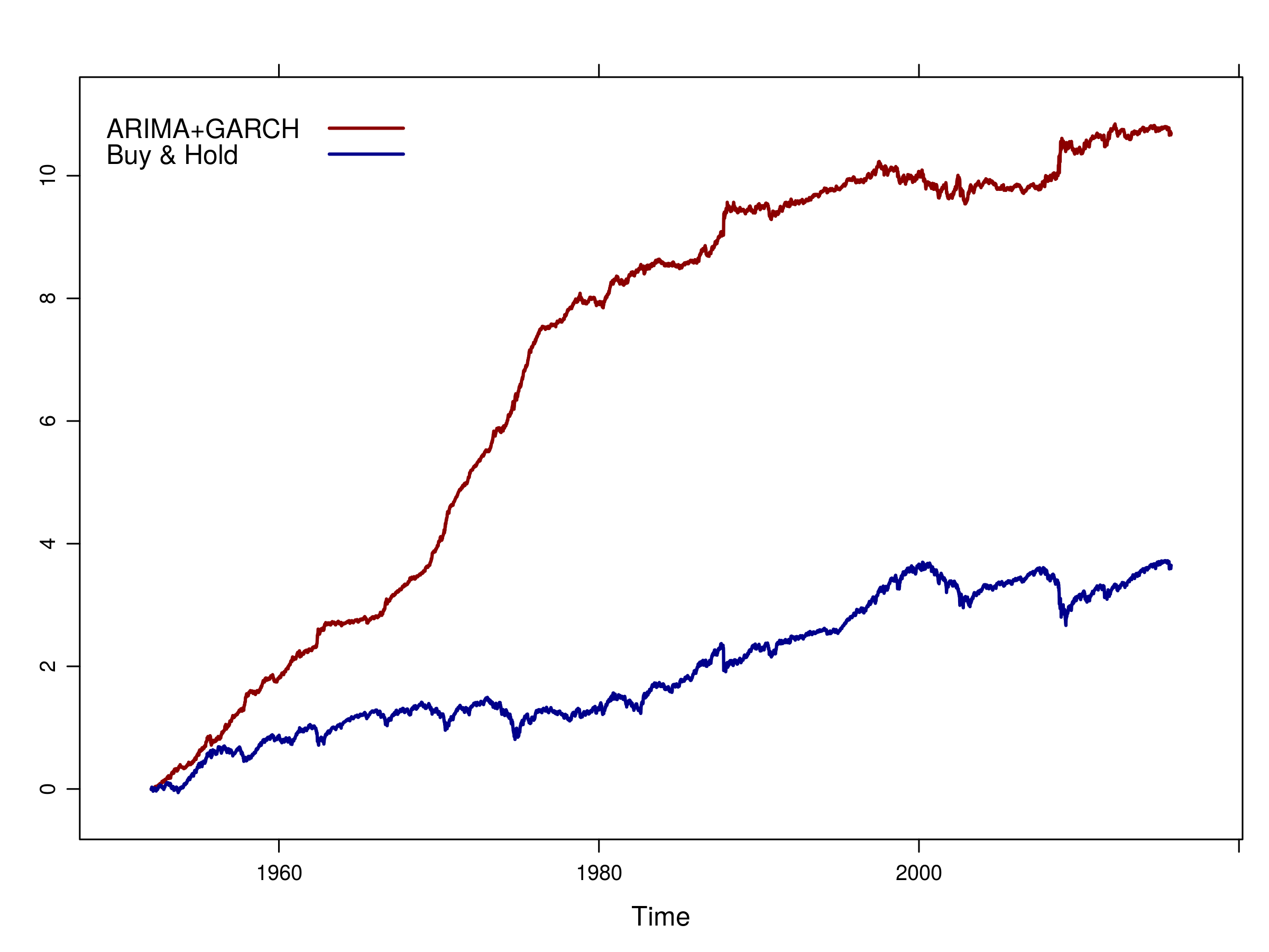 Equity curve of ARIMA+GARCH strategy vs "Buy & Hold" for the S&P500 from 1952
As you can see, over a 65 year period, the ARIMA+GARCH strategy has significantly outperformed "Buy & Hold". However, you can also see that the majority of the gain occured between 1970 and 1980. Notice that the volatility of the curve is quite minimal until the early 80s, at which point the volatility increases significantly and the average returns are less impressive.
Clearly the equity curve promises great performance over the whole period. However, would this strategy really have been tradeable?
First of all, let's consider the fact that the ARMA model was only published in 1951. It wasn't really widely utilised until the 1970's when Box & Jenkins discussed it in their book.
Secondly, the ARCH model wasn't discovered (publicly!) until the early 80s, by Engle, and GARCH itself was published by Bollerslev in 1986.
Thirdly, this "backtest" has actually been carried out on a stock market index and not a physically tradeable instrument. In order to gain access to an index such as this it would have been necessary to trade S&P500 futures or a replica Exchange Traded Fund (ETF) such as SPDR.
Hence is it really that appropriate to apply such models to a historical series prior to their invention? An alternative is to begin applying the models to more recent data. In fact, we can consider the performance in the last ten years, from Jan 1st 2005 to today:
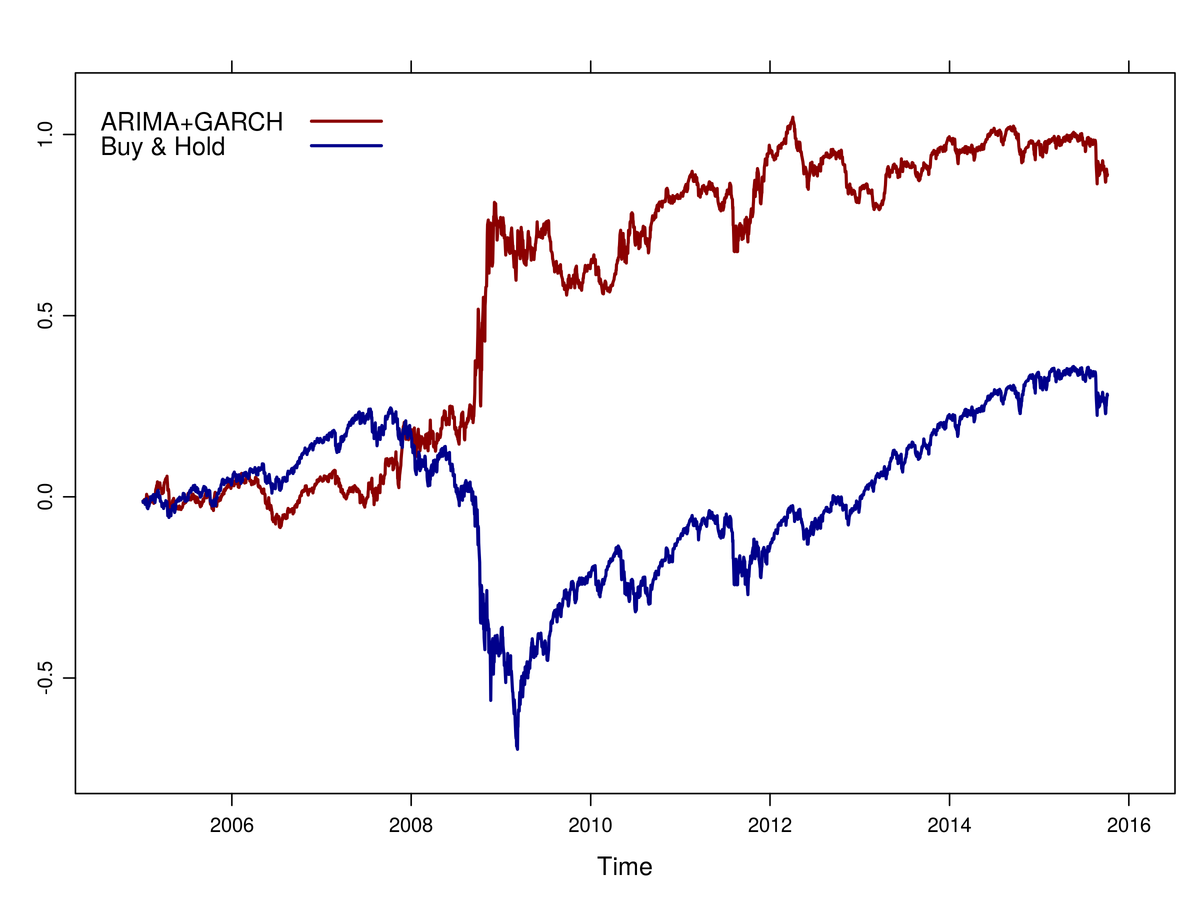 Equity curve of ARIMA+GARCH strategy vs "Buy & Hold" for the S&P500 from 2005 until today
As you can see the equity curve remains below a Buy & Hold strategy for almost 3 years, but during the stock market crash of 2008/2009 it does exceedingly well. This makes sense because there is likely to be a significant serial correlation in this period and it will be well-captured by the ARIMA and GARCH models. Once the market recovered post-2009 and enters what looks to be more a stochastic trend, the model performance begins to suffer once again.
Note that this strategy can be easily applied to different stock market indices, equities or other asset classes. I strongly encourage you to try researching other instruments, as you may obtain substantial improvements on the results presented here.
Next Steps
Now that we've finished discussing the ARIMA and GARCH family of models, I want to continue the time series analysis discussion by considering long-memory processes, state-space models and cointegrated time series.
These subsequent areas of time series will introduce us to models that can improve our forecasts beyond those I've presented here, which will significantly increase our trading profitability and/or reduce risk.
Full Code
Here is the full listing for the indicator generation, backtesting and plotting:
# Import the necessary libraries
library(quantmod)
library(lattice)
library(timeSeries)
library(rugarch)

# Obtain the S&P500 returns and truncate the NA value
getSymbols("^GSPC", from="1950-01-01")
spReturns = diff(log(Cl(GSPC)))
spReturns[as.character(head(index(Cl(GSPC)),1))] = 0

# Create the forecasts vector to store the predictions
windowLength = 500
foreLength = length(spReturns) - windowLength
forecasts <- vector(mode="character", length=foreLength)

for (d in 0:foreLength) {
    # Obtain the S&P500 rolling window for this day
    spReturnsOffset = spReturns[(1+d):(windowLength+d)]

    # Fit the ARIMA model
    final.aic <- Inf
    final.order <- c(0,0,0)
    for (p in 0:5) for (q in 0:5) {
        if ( p == 0 && q == 0) {
            next
        }

        arimaFit = tryCatch( arima(spReturnsOffset, order=c(p, 0, q)),
                             error=function( err ) FALSE,
                             warning=function( err ) FALSE )

        if( !is.logical( arimaFit ) ) {
            current.aic <- AIC(arimaFit)
            if (current.aic < final.aic) {
                final.aic <- current.aic
                final.order <- c(p, 0, q)
                final.arima <- arima(spReturnsOffset, order=final.order)
            }
        } else {
            next
        }
    }

    # Specify and fit the GARCH model
    spec = ugarchspec(
        variance.model=list(garchOrder=c(1,1)),
        mean.model=list(armaOrder=c(final.order[1], final.order[3]), include.mean=T),
        distribution.model="sged"
    )
    fit = tryCatch(
      ugarchfit(
        spec, spReturnsOffset, solver = 'hybrid'
      ), error=function(e) e, warning=function(w) w
    )

    # If the GARCH model does not converge, set the direction to "long" else
    # choose the correct forecast direction based on the returns prediction
    # Output the results to the screen and the forecasts vector
    if(is(fit, "warning")) {
      forecasts[d+1] = paste(index(spReturnsOffset[windowLength]), 1, sep=",")
      print(paste(index(spReturnsOffset[windowLength]), 1, sep=","))
    } else {
      fore = ugarchforecast(fit, n.ahead=1)
      ind = fore@forecast$seriesFor
      forecasts[d+1] = paste(colnames(ind), ifelse(ind[1] < 0, -1, 1), sep=",")
      print(paste(colnames(ind), ifelse(ind[1] < 0, -1, 1), sep=","))
    }
}

# Output the CSV file to "forecasts.csv"
write.csv(forecasts, file="forecasts.csv", row.names=FALSE)

# Input the Python-refined CSV file
spArimaGarch = as.xts(
  read.zoo(
    file="forecasts_new.csv", format="%Y-%m-%d", header=F, sep=","
  )
)

# Create the ARIMA+GARCH returns
spIntersect = merge( spArimaGarch[,1], spReturns, all=F )
spArimaGarchReturns = spIntersect[,1] * spIntersect[,2]

# Create the backtests for ARIMA+GARCH and Buy & Hold
spArimaGarchCurve = log( cumprod( 1 + spArimaGarchReturns ) )
spBuyHoldCurve = log( cumprod( 1 + spIntersect[,2] ) )
spCombinedCurve = merge( spArimaGarchCurve, spBuyHoldCurve, all=F )

# Plot the equity curves
xyplot(
  spCombinedCurve,
  superpose=T,
  col=c("darkred", "darkblue"),
  lwd=2,
  key=list(
    text=list(
      c("ARIMA+GARCH", "Buy & Hold")
    ),
    lines=list(
      lwd=2, col=c("darkred", "darkblue")
    )
  )
)
And the Python code to apply to forecasts.csv before reimporting:
forecasts = open("forecasts.csv", "r").readlines()

old_value = 1
new_list = []
for f in forecasts[1:]:
    strpf = f.replace('"','').strip()
    new_str = "%s,%s\n" % (strpf, old_value)
    newspl = new_str.strip().split(",")
    final_str = "%s,%s\n" % (newspl[0], newspl[2])
    final_str = final_str.replace('"','')
    old_value = f.strip().split(',')[1]
    new_list.append(final_str)

out = open("forecasts_new.csv", "w")
for n in new_list:
    out.write(n)


