Tutorial: 60/40 Portfolio

In this basic tutorial we are going to demonstrate some of QSTrader's functionality by backtesting a simple 60/40 US Equities/Bonds benchmark strategy. The tutorial assumes you have correctly installed QSTrader.

Please note that all of the code below can be found within the /examples/sixty_forty.py file at the QSTrader GitHub repository. We will be referring to this file in the tutorial steps below.

The first task is to either download the sixty_forty.py file, utilise the full code at the end of this tutorial or create a new empty file to type in the code below manually.

We will begin by describing the strategy and download the necessary data from Yahoo Finance. We will subsequently describe all code in sixty_forty.py and finally execute the backtest to display a performance 'tearsheet'.

Strategy Explanation

The 60/40 US Equities/Bonds strategy is a simple long-term investment approach that is widely utilised in the investment industry. It seeks to ensure that at any point during the lifetime of the investment that 60% of account equity is invested in one or more assets representing a broad selection of US equities (such as an S&P500 ETF), while 40% of account equity is invested in one or more assets representing a broad selection of US treasury bonds (such as a treasury bond ETF).

Since the actual percentage allocations of each asset class can deviate over time due to relative growth of the respective assets a 'rebalance' approach is often carried out. This means that trades are issued on a relatively infrequent basis to buy/sell amounts of each asset class to periodically bring the account equity allocations back into the 60/40 split. For the particular strategy implemented here we are using an end of month rebalance frequency.

We have written a more detailed article on the 60/40 benchmark which you can read here.

Downloading the Data

The sixty_forty.py code makes use of OHLC 'daily bar' data from Yahoo Finance. In particular it requires the SPY and AGG ETFs data. Download the full history for each and save as CSV files in same directory as sixty_forty.py.

Defining a Backtest Script

Module Imports

The first part of the Python code imports the necessary modules from within the QSTrader library:

# sixty_forty.py

import os

import pandas as pd
import pytz

from qstrader.alpha_model.fixed_signals import FixedSignalsAlphaModel
from qstrader.asset.equity import Equity
from qstrader.asset.universe.static import StaticUniverse
from qstrader.data.backtest_data_handler import BacktestDataHandler
from qstrader.data.daily_bar_csv import CSVDailyBarDataSource
from qstrader.statistics.tearsheet import TearsheetStatistics
from qstrader.trading.backtest import BacktestTradingSession

We first import os as we need to query the environment for the appropriate QSTrader data directory. It is possible to tell QSTrader to look for data in a directory other than the same directory as the sixty_forty.py file, but for the purposes of this tutorial we will assume the data will eventually be stored in the same directory.

We then import Pandas and Pytz, which are needed for handling timestamp functionality with timezones.

The remaining imports are within QSTrader itself. We first import a FixedSignalsAlphaModel. An AlphaModel in QSTrader terms is a class that emits a dimensionless 'forecast' or 'signal' for a particular collection of assets (known as an 'asset universe').

The FixedSignalsAlphaModel is a simple signal generator that emits constant forecasts, irrespective of market behaviour for a particular collection of assets. Since we are targeting a 60%/40% split of US equities/bonds our signals will remain constant throughout the backtest lifetime at 0.6 for SPY and 0.4 for AGG.

We import Equity in order to tell the module that loads the data from CSV files that the CSV files represent equity prices/volumes.

We import the StaticUniverse class because our asset 'universe' consists solely of the SPY and AGG ETFs and will not change through time.

We import the helper BacktestDataHandler class that determines how our asset universe specification and data source(s) are linked.

We import the CSVDailyBarDataSource because the particular data sources used within this tutorial are CSV files, as opposed to a database, web URL or file store (such as HDF5).

Since we wish to visualise our backtest results we want to import the TearsheetStatistics class.

Finally to tie it all together we import the BacktestTradingSession, which runs our scheduled backtest 'engine' between the specified start and end timestamps.

Backtest Duration

The next task is to define the script entry point and specify when the backtest runs from and to:

# sixty_forty.py

if __name__ == "__main__":
    start_dt = pd.Timestamp('2003-09-30 14:30:00', tz=pytz.UTC)
    end_dt = pd.Timestamp('2019-12-31 23:59:00', tz=pytz.UTC)

Note that the dates make use of the Pandas Timestamp class and require timezone specification.

Also please note that at this stage of QSTrader development, for the 'buy & hold' methodology used below it is necessary to specify a starting time of 14:30:00 UTC in order for the backtest to proceed correctly.

Asset Universe

The next task is to construct the universe for the backtest:

# sixty_forty.py

    # Construct the symbols and assets necessary for the backtest
    strategy_symbols = ['SPY', 'AGG']
    strategy_assets = ['EQ:%s' % symbol for symbol in strategy_symbols]
    strategy_universe = StaticUniverse(strategy_assets)

QSTrader requires that the assets are prefixed with a two letter code describing their instrument type. In this simulation the assets must be prefixed with EQ, representing equity-like (common stock and ETFs) instruments. Finally a StaticUniverse is instantiated with the appropriate assets.

Pricing Data

The next task is to obtain the appropriate data for these symbols and load it into the data handler:

# sixty_forty.py

    # To avoid loading all CSV files in the directory, set the
    # data source to load only those provided symbols
    csv_dir = os.environ.get('QSTRADER_CSV_DATA_DIR', '.')
    data_source = CSVDailyBarDataSource(csv_dir, Equity, csv_symbols=strategy_symbols)
    data_handler = BacktestDataHandler(strategy_universe, data_sources=[data_source])

Firstly we determine the appropriate data directory if it has been set externally by the environment, otherwise we default to the same directory as sixty_forty.py. Then we load the CSV data and tie it together with the asset universe through a BacktestDataHandler.

Alpha Model and Backtest

The next set of code creates the alpha model, defines the backtest and executes it:

# sixty_forty.py

    # Construct an Alpha Model that simply provides
    # static allocations to a universe of assets
    # In this case 60% SPY ETF, 40% AGG ETF,
    # rebalanced at the end of each month
    strategy_alpha_model = FixedSignalsAlphaModel({'EQ:SPY': 0.6, 'EQ:AGG': 0.4})
    strategy_backtest = BacktestTradingSession(
        start_dt,
        end_dt,
        strategy_universe,
        strategy_alpha_model,
        rebalance='end_of_month',
        long_only=True,
        cash_buffer_percentage=0.01,
        data_handler=data_handler
    )
    strategy_backtest.run()

Firstly the FixedSignalsAlphaModel is initialised with a dictionary containing assets as keys and their lifetime fixed signals as values. This represents a 60% target allocation to the SPY ETF and a 40% target allocation to the AGG ETF.

Subsequently the BacktestTradingSession is initialised with the start/end dates, the asset universe and the particular alpha model defined above.

In addition it is necessary to supply a rebalance keyword argument. This tells the QSTrader backtesting engine how frequently to re-run the signal generation and portfolio construction logic. Since this is decoupled from the actual data timestamps it is necessary to be explicit about how frequently this is carried out.

For this particular strategy we are going to carry out the signal generation and portfolio construction once per month at the close of the final trading day. This means that if the true percentage allocations of SPY and AGG have drifted from their 60% and 40% allocations across the month some additional 'rebalance' trades will be issued to buy/sell the appropriate amount of stock in order to bring the account allocations inline with these targets.

The long_only keyword argument lets the backtester know that this strategy only goes 'long' (that is, does not borrow and 'short' any assets on margin).

We also require a 'cash buffer' in the account in order to handle the case where a target order for a particular quantity of stock is generated (at market close) but when executed at the next market open the order is found to be too expensive for the current account equity to execute.

This can occur if the stock price for this asset has jumped up significantly overnight. This cash buffer attempts to account for such jumps. It maintains this (approximate) percentage of the account equity in cash to cover this eventuality. We have set it to 1% of account equity here but it may be necessary to modify this value if backtesting on particularly volatile equities.

Finally we tell the backtesting engine which data handler to use and execute the backtest with the run method.

At this stage, once the backtest has finished executing the strategy_backtest instance contains all of the calculated values of the backtest (such as the equity curve, drawdown curve and various other statistics).

Benchmark

However we are also interested in comparing this result to another 'benchmark' strategy, which is simply a 'buy & hold' of the SPY ETF. This allows to see what has happened over the backtest duration if we simply held onto stocks during this time period, rather than a 60/40 allocation to stocks/bonds.

To create a benchmark we run another full backtest, but on a slightly different alpha model and rebalance schedule:

# sixty_forty.py

    # Construct a benchmark Alpha Model that provides
    # 100% static allocation to the SPY ETF, with no rebalance
    benchmark_alpha_model = FixedSignalsAlphaModel({'EQ:SPY': 1.0})
    benchmark_backtest = BacktestTradingSession(
        start_dt,
        end_dt,
        benchmark_universe,
        benchmark_alpha_model,
        rebalance='buy_and_hold',
        long_only=True,
        cash_buffer_percentage=0.01,
        data_handler=data_handler
    )
    benchmark_backtest.run()

Note that the FixedSignalsAlphaModel has a 100% allocation to SPY for the benchmark. It also uses the 'buy_and_hold' rebalance schedule. The latter informs the backtester to generate a single signal at the beginning of the backtest to go fully long SPY. There are no further trades carried out for the benchmark.

The remaining parameters are similar and we run the benchmark backtest once again with the run method.

Tearsheet

All of the backtest results are now stored in strategy_backtest and benchmark_backtest. However we would like to visualise these results and output some basic statistics. For this we can use a 'tearsheet':

# sixty_forty.py

    # Performance Output
    tearsheet = TearsheetStatistics(
        strategy_equity=strategy_backtest.get_equity_curve(),
        benchmark_equity=benchmark_backtest.get_equity_curve(),
        title='60/40 US Equities/Bonds'
    )
    tearsheet.plot_results()

The TearsheetStatistics class is instantiated with the strategy backtest equity curve, the (optional) benchmark backtest equity curve and a supplied title. Finally the results are plotted (using Matplotlib) through the plot_results method.

Executing the Backtest

To run the code ensure that your Python virtual environment, such as Anaconda or virtualenv is activated. Then type the following in the same directory as sixty_forty.py:

python sixty_forty.py

You will see both the strategy and benchmark backtests being calculated. Finally the tearsheet will appear depicting the results. It should look like the following:

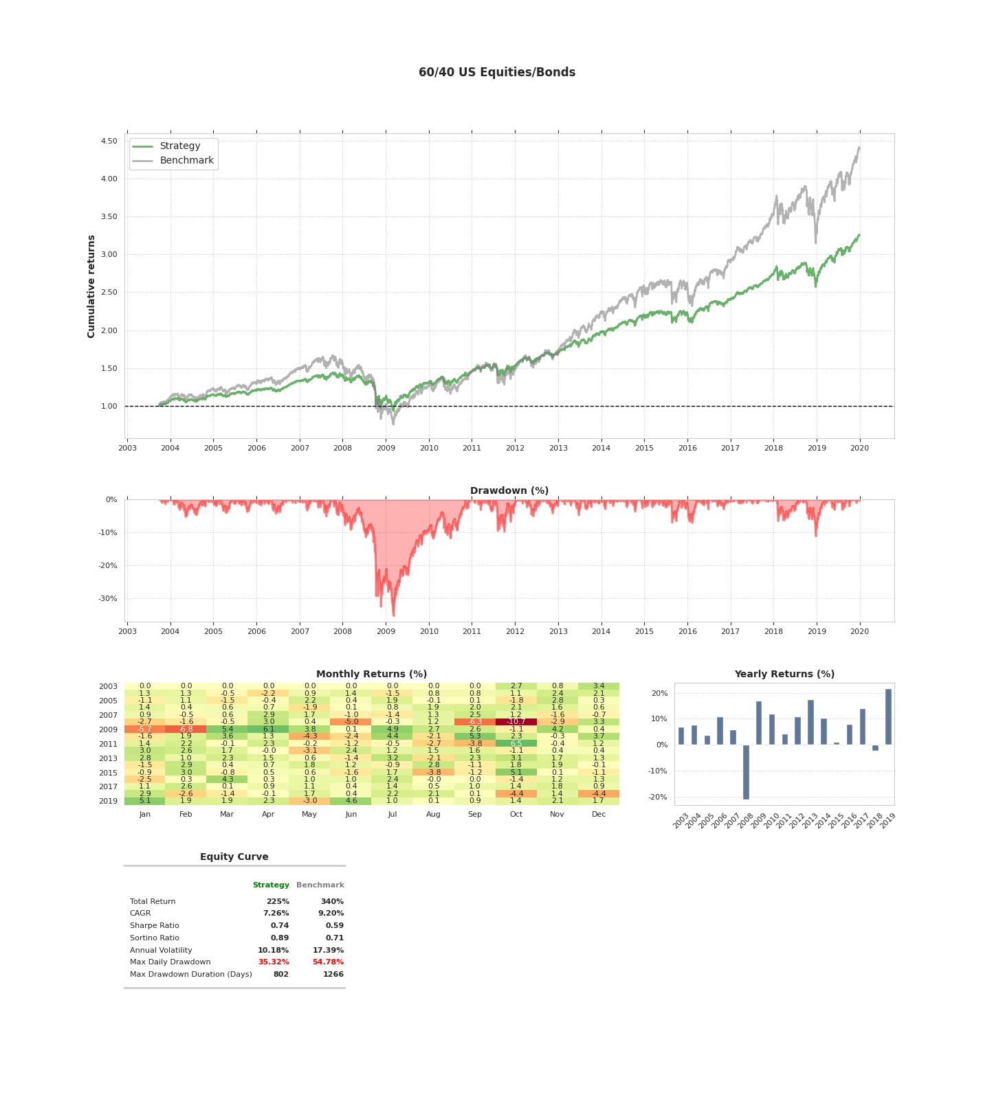
You have now successfully completed your first QSTrader backtest!

Full Code

import os

import pandas as pd
import pytz

from qstrader.alpha_model.fixed_signals import FixedSignalsAlphaModel
from qstrader.asset.equity import Equity
from qstrader.asset.universe.static import StaticUniverse
from qstrader.data.backtest_data_handler import BacktestDataHandler
from qstrader.data.daily_bar_csv import CSVDailyBarDataSource
from qstrader.statistics.tearsheet import TearsheetStatistics
from qstrader.trading.backtest import BacktestTradingSession


if __name__ == "__main__":
    start_dt = pd.Timestamp('2003-09-30 14:30:00', tz=pytz.UTC)
    end_dt = pd.Timestamp('2019-12-31 23:59:00', tz=pytz.UTC)

    # Construct the symbols and assets necessary for the backtest
    strategy_symbols = ['SPY', 'AGG']
    strategy_assets = ['EQ:%s' % symbol for symbol in strategy_symbols]
    strategy_universe = StaticUniverse(strategy_assets)

    # To avoid loading all CSV files in the directory, set the
    # data source to load only those provided symbols
    csv_dir = os.environ.get('QSTRADER_CSV_DATA_DIR', '.')
    data_source = CSVDailyBarDataSource(csv_dir, Equity, csv_symbols=strategy_symbols)
    data_handler = BacktestDataHandler(strategy_universe, data_sources=[data_source])

    # Construct an Alpha Model that simply provides
    # static allocations to a universe of assets
    # In this case 60% SPY ETF, 40% AGG ETF,
    # rebalanced at the end of each month
    strategy_alpha_model = FixedSignalsAlphaModel({'EQ:SPY': 0.6, 'EQ:AGG': 0.4})
    strategy_backtest = BacktestTradingSession(
        start_dt,
        end_dt,
        strategy_universe,
        strategy_alpha_model,
        rebalance='end_of_month',
        long_only=True,
        cash_buffer_percentage=0.01,
        data_handler=data_handler
    )
    strategy_backtest.run()

    # Construct benchmark assets (buy & hold SPY)
    benchmark_assets = ['EQ:SPY']
    benchmark_universe = StaticUniverse(benchmark_assets)

    # Construct a benchmark Alpha Model that provides
    # 100% static allocation to the SPY ETF, with no rebalance
    benchmark_alpha_model = FixedSignalsAlphaModel({'EQ:SPY': 1.0})
    benchmark_backtest = BacktestTradingSession(
        start_dt,
        end_dt,
        benchmark_universe,
        benchmark_alpha_model,
        rebalance='buy_and_hold',
        long_only=True,
        cash_buffer_percentage=0.01,
        data_handler=data_handler
    )
    benchmark_backtest.run()

    # Performance Output
    tearsheet = TearsheetStatistics(
        strategy_equity=strategy_backtest.get_equity_curve(),
        benchmark_equity=benchmark_backtest.get_equity_curve(),
        title='60/40 US Equities/Bonds'
    )
    tearsheet.plot_results()