We have spent a good deal of time looking at vanilla and path-dependent options on QuantStart so far. We have created separate classes for random number generation and sampling from a standard normal distribution. We're now going to build on this by generating correlated time series paths.
Correlated asset paths crop up in many areas of quantitative finance and options pricing. In particular, the Heston Stochastic Volatility Model requires two correlated GBM asset paths as a basis for modelling volatility.
Motivation
Let's motivate the generation of correlated asset paths via the Heston Model. The original Black-Scholes model assumes that volatility, $\sigma$, is constant over the lifetime of the option, leading to the stochastic differential equation (SDE) for GBM (using the Wikipedia notation):
\begin{eqnarray} dS_t = \mu S_t dt + \sigma S_t dW_t \end{eqnarray}The basic Heston model now replaces the constant $\sigma$ coefficient with the square root of the instantaneous variance, $\sqrt{\nu_t}$. Thus the full model is given by:
\begin{eqnarray} dS_t &=& \mu S_t dt + \sqrt{\nu_t} S_t dW^S_t \\ d\nu_t &=& \kappa(\theta - \nu_t) dt + \xi \sqrt{\nu_t} dW^{\nu}_t \end{eqnarray}Where $dW^S_t$ and $dW^{\nu}_t$ are Brownian motions with correlation $\rho$. Hence we have two correlated stochastic processes. In order to price path-dependent options in the Heston framework by Monte Carlo, it is necessary to generate these two asset paths.
Process for Correlated Path Generation
Rather than considering the case of two correlated assets, we will look at $N$ seperate assets and then reduce the general procedure to $N=2$ for the case of our Heston motivating example. This reminds me of an old mathematics joke*.
At each time step in the path generation we require $N$ correlated random numbers, where $\rho_{ij}$ denotes the correlation coefficient between the $i$th and $j$th asset, $x_i$ will be the uncorrelated random number (which we will sample from the standard normal distribution), $\epsilon_i$ will be a correlated random number, used in the asset path generation and $\alpha_{ij}$ will be a matrix coefficient necessary for obtaining $\epsilon_i$.
To calculate $\epsilon_i$ we use the following process for each of the path generation time-steps:
\begin{eqnarray} \epsilon_i = \sum^{i}_{k=1} \alpha_{ik} x_k, 1 \leq i \leq N \\ \sum^{i}_{k=1} \alpha^2_{ik} = 1, 1 \leq i \leq N \\ \sum^{i}_{k=1} \alpha_{ik} \alpha_{jk} = \rho_{ij}, \forall j < i \end{eqnarray}Thankfully, for our Heston model, we have $N=2$ and this reduces the above equation set to the far simpler relations:
\begin{eqnarray} \epsilon_1 &=& x_1 \\ \epsilon_2 &=& \rho x_1 + x_2 \sqrt{1 - \rho^2} \end{eqnarray}This motivates a potential C++ implementation. We already have the capability to generate paths of standard normal distributions. If we inherit a new class CorrelatedSND (SND for 'Standard Normal Distribution'), we can provide it with a correlation coefficient and an original time series of random standard normal variables draws to generate a new correlated asset path.
Cholesky Decomposition
It can be seen that the process used to generate $N$ correlated $\epsilon_i$ values is in fact a matrix equation. It turns out that it is actually a Cholesky Decomposition, which I have written about before (albeit in a Python context).
Thus a far more efficient implementation than I am constructing here would make use of an optimised matrix class and a pre-computed Cholesky decomposition matrix.
The reason for this link is that the correlation matrix, $\Sigma$, is symmetric positive definite. Thus it can be decomposed into $\Sigma = RR^{*}$, although $R^{*}$, the conjugate-transpose matrix simply reduces to the transpose in the case of real-valued entries, with $R$ a lower-triangular matrix.
Hence it is possible to calculate the correlated random variable vector ${\bf \epsilon}$ via:
\begin{eqnarray} {\bf \epsilon} = {\bf R} {\bf x} \end{eqnarray}Where ${\bf x}$ is the vector of uncorrelated variables.
We will explore the Cholesky Decomposition as applied to multiple correlated asset paths in later articles.
C++ Implementation
As we pointed out above the procedure for obtaining the second path will involve calculating an uncorrelated set of standard normal draws, which are then recalculated via an inherited subclass to generate a new, correlated set of random variables. For this we will make use of statistics.h and statistics.cpp, which can be found in the article on statistical distributions in C++.
Our next task is to write the header and source files for CorrelatedSND. The listing for correlated_snd.h follows:
#ifndef __CORRELATED_SND_H
#define __CORRELATED_SND_H

#include "statistics.h"

class CorrelatedSND : public StandardNormalDistribution {
 protected:
  double rho;
  const std::vector<double>* uncorr_draws;

  // Modify an uncorrelated set of distribution draws to be correlated
  virtual void correlation_calc(std::vector<double>& dist_draws);

 public:
  CorrelatedSND(const double _rho,
                const std::vector<double>* _uncorr_draws);
  virtual ~CorrelatedSND();

  // Obtain a sequence of correlated random draws from another set of SND draws
  virtual void random_draws(const std::vector<double>& uniform_draws,
                            std::vector<double>& dist_draws);
};

#endif
The class inherits from StandardNormalDistribution, provided in statistcs.h. We are adding two protected members, rho (the correlation coefficient) and uncorr_draws, a pointer to a const vector of doubles. We also create an additional virtual method, correlation_calc, that actually performs the correlation calculation. The only additional modification is to add the parameters, which will ultimately become stored as protected member data, to the constructor.
Next up is the source file, correlated_snd.cpp:
#ifndef __CORRELATED_SND_CPP
#define __CORRELATED_SND_CPP

#include "correlated_snd.h"
#include <iostream>
#include <cmath>

CorrelatedSND::CorrelatedSND(const double _rho,
                         const std::vector<double>* _uncorr_draws)
  : rho(_rho), uncorr_draws(_uncorr_draws) {}

CorrelatedSND::~CorrelatedSND() {}

// This carries out the actual correlation modification. It is easy to see that if
// rho = 0.0, then dist_draws is unmodified, whereas if rho = 1.0, then dist_draws
// is simply set equal to uncorr_draws. Thus with 0 < rho < 1 we have a
// weighted average of each set.
void CorrelatedSND::correlation_calc(std::vector<double>& dist_draws) {
    for (int i=0; i<dist_draws.size(); i++) {
      dist_draws[i] = rho * (*uncorr_draws)[i] + dist_draws[i] * sqrt(1-rho*rho);
    }
}

void CorrelatedSND::random_draws(const std::vector<double>& uniform_draws,
                                 std::vector<double>>& dist_draws) {
  // The following functionality is lifted directly from
  // statistics.h, which is fully commented!
  if (uniform_draws.size() != dist_draws.size()) {
    std::cout << "Draws vectors are of unequal size in standard normal dist." << std::endl;
    return;
  }

  if (uniform_draws.size() % 2 != 0) {
    std::cout << "Uniform draw vector size not an even number." << std::endl;
    return;
  }

  for (int i=0; i<uniform_draws.size() / 2; i++) {
    dist_draws[2*i] = sqrt(-2.0*log(uniform_draws[2*i])) * sin(2*M_PI*uniform_draws[2*i+1]);
    dist_draws[2*i+1] = sqrt(-2.0*log(uniform_draws[2*i])) * cos(2*M_PI*uniform_draws[2*i+1]);
  }

  // Modify the random draws via the correlation calculation
  correlation_calc(dist_draws);

  return;
}

#endif
The work is carried out in correlation_calc. It is easy to see that if $\rho = 0$, then dist_draws is unmodified, whereas if $\rho = 1$, then dist_draws is simply equated to uncorr_draws. Thus with $0 < \rho < 1$ we have a weighted average of each set of random draws. Note that I have reproduced the Box-Muller functionality here so that you don't have to look it up in statistics.cpp. In a production code this would be centralised elsewhere (such as with a random number generator class).
Now we can tie it all together. Here is the listing of main.cpp:
#include "statistics.h"
#include "correlated_snd.h"
#include <iostream>
#include <vector>

int main(int argc, char **argv) {

  // Number of values
  int vals = 30;

  /* UNCORRELATED SND */
  /* ================ */

  // Create the Standard Normal Distribution and random draw vectors
  StandardNormalDistribution snd;
  std::vector<double> snd_uniform_draws(vals, 0.0);
  std::vector<double> snd_normal_draws(vals, 0.0);

  // Simple random number generation method based on RAND
  // We could be more sophisticated an use a LCG or Mersenne Twister
  // but we're trying to demonstrate correlation, not efficient
  // random number generation!
  for (int i=0; i<snd_uniform_draws.size(); i++) {
    snd_uniform_draws[i] = rand() / static_cast<double>(RAND_MAX);
  }

  // Create standard normal random draws
  snd.random_draws(snd_uniform_draws, snd_normal_draws);

  /* CORRELATION SND */
  /* =============== */

  // Correlation coefficient
  double rho = 0.5;

  // Create the correlated standard normal distribution
  CorrelatedSND csnd(rho, &snd_normal_draws);
  std::vector<double> csnd_uniform_draws(vals, 0.0);
  std::vector<double> csnd_normal_draws(vals, 0.0);

  // Uniform generation for the correlated SND
  for (int i=0; i<csnd_uniform_draws.size(); i++) {
    csnd_uniform_draws[i] = rand() / static_cast<double>(RAND_MAX);
  }

  // Now create the -correlated- standard normal draw series
  csnd.random_draws(csnd_uniform_draws, csnd_normal_draws);

  // Output the values of the standard normal random draws
  for (int i=0; i<snd_normal_draws.size(); i++) {
    std::cout << snd_normal_draws[i] << ", " << csnd_normal_draws[i] << std::endl;
  }

  return 0;
}
The above code is somewhat verbose, but that is simply a consequence of not encapsulating the random number generation capability. Once we have created an initial set of standard normal draws, we simply have to pass that to an instance of CorrelatedSND (in this line: CorrelatedSND csnd(rho, &snd_normal_draws);) and then call random_draws(..) to create the correlated stream. Finally, we output both sets of values:
3.56692, 1.40915
3.28529, 1.67139
0.192324, 0.512374
-0.723522, 0.992231
1.10093, 1.14815
0.217484, -0.211253
-2.22963, -1.94287
-1.06868, -0.500967
-0.35082, -0.0884041
0.806425, 0.326177
-0.168485, -0.242706
-1.3742, 0.752414
0.131154, -0.632282
0.59425, 0.311842
-0.449029, 0.129012
-2.37823, -0.469604
0.0431789, -0.52855
0.891999, 1.0677
0.564585, 0.825356
1.26432, -0.653957
-1.21881, -0.521325
-0.511385, -0.881099
-0.43555, 1.23216
0.93222, 0.237333
-0.0973298, 1.02387
-0.569741, 0.33579
-1.7985, -1.52262
-1.2402, 0.211848
-1.26264, -0.490981
-0.39984, 0.150902
Here is a plot of the two time series:
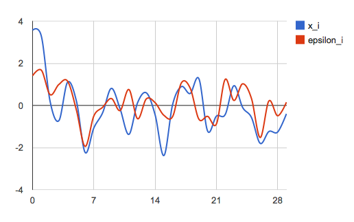
Two standard normal distribution random draw time series with correlation $\rho = 0.5$
There are plenty of extensions we could make to this code. The obvious two are encapsulating the random number generation and converting it to use an efficient Cholesky Decomposition implementation. Now that we have correlated streams, we can also implement the Heston Model in Monte Carlo.
* A mathematician and his best friend, an engineer, attend a public lecture on geometry in thirteen-dimensional space. "How did you like it?" the mathematician wants to know after the talk. "My head's spinning", the engineer confesses. "How can you develop any intuition for thirteen-dimensional space?". "Well, it's not even difficult. All I do is visualize the situation in arbitrary N-dimensional space and then set N = 13."


