Over the last ten years the subject of deep learning has been one of the most discussed fields in machine learning and artificial intelligence. It has produced state-of-the-art results in areas as diverse as computer vision, image recognition, natural language processing and speech recognition. However it has also been widely hyped - the answer to all machine learning problems - and is often misunderstood due to its steep learning curve.
In the last couple of years one of the leading deep learning firms, Google DeepMind, has managed to use a particular technique known as deep reinforcement learning to beat humans at Atari 2600 games[7]. In a highly-publicised recent contest[8] the AlphaGo model beat the top-ranked Go player over a number of games, further enhancing the mystery and excitement surrounding this machine learning technique.
Deep learning is not an easy subject to learn and requires some undergraduate mathematical prerequisites in order to get started. In particular one should be familiar with the basic elements of linear algebra, vector calculus (gradients, partial derivatives) and probability (maximum likelihood estimation). In addition to the mathematical prerequisites it requires a good understanding of object-oriented programming and, for efficiency purposes, a basic familiarity with the operations of a GPU. However we will try and introduce many of these concepts as they are needed. Hence the article series should be relatively self-contained for those with some mathematical background.
In these articles we are going to find out what deep learning is, why it has recently become so popular, how it works and how we can apply it to areas of quantitative finance in order to improve our model results and portfolio profitability. We will make use of a Python library called Theano[5] and GPUs, which will provide significant increases in training performance.
In particular we are going to consider the following topics over the course of the series:
- Logistic Regression in Theano (this article)
- Neural Networks and the Multilayer Perceptron
- Convolution Neural Networks (ConvNets)
- Denoising Autoencoders and Stacked Denoising Autoencoders
- Restricted Boltzmann Machines
- Deep Belief Networks
- Reinforcement Learning and Q-Learning
- Deep Learning for Time Series Analysis
Note: If you think you might struggle with the mathematical prerequisites for this article series you should take a look at Part 1 and Part 2 of the "How to Learn Mathematics Without Heading to University" articles to brush up on your mathematics.
What is Deep Learning?
Deep learning is a subset of the larger field of machine learning that attempts to model high level abstractions in data in order to vastly improve performance in both supervised and unsupervised learning[9].
It achieves this by using multiple layers of "processors", each of which contains a set of non-linear transformation functions that learn representations within the data.
Such an approach is motivated directly by how the brain is thought to work. Over the course of our lifetime we learn about simple ideas and then use these simple ideas to form hierarchies of more complex ideas. Deep learning is about applying this approach to machine learning tasks.
General Motivation for Deep Learning
One of the major problems with statistical machine learning is that it often requires a great deal of time to hand craft features, or predictors, in order to generate effective classification or regression algorithms. For instance, when attempting to predict future values of an equity market index it might be pertinent to include interest rates, commodities prices or equity fundamental data. Or for data that is initially not in a convenient numerical representation such as video, audio or text it is necessary to find efficient transformation algorithms to produce predictive features.
Choosing optimal features is difficult and time consuming. Features often need to be handcrafted via dimensionality reduction or transformation in order to improve predictive performance. Examples of such transformations include the bag of words and term frequency-inverse document frequency vectorisation methods for natural language processing.
Deep learning promises to replace the time-consuming task of handcrafted feature engineering via the introduction of efficient network architectures for unsupervised feature learning. The key to this process lies in the hierarchical representation of features within the network structure.
Current research into deep learning algorithms attempts to create models that learn abstract representations from vast quantities of unlabeled data. This is because unlabeled data is often extremely abundant compared to the more costly process of obtaining labeled data, the latter of which is used for supervised learning approaches.
Deep learning has become popular over the last ten years due in part to a set of three "breakthrough" papers by Geoff Hinton, Yoshua Bengio, Yann LeCun and others[2]:
- Hinton, G. E., Osindero, S. and Teh, Y., A fast learning algorithm for deep belief nets Neural Computation 18:1527-1554, 2006
- Yoshua Bengio, Pascal Lamblin, Dan Popovici and Hugo Larochelle, Greedy Layer-Wise Training of Deep Networks, in J. Platt et al. (Eds), Advances in Neural Information Processing Systems 19 (NIPS 2006), pp. 153-160, MIT Press, 2007
- Marc’Aurelio Ranzato, Christopher Poultney, Sumit Chopra and Yann LeCun Efficient Learning of Sparse Representations with an Energy-Based Model, in J. Platt et al. (Eds), Advances in Neural Information Processing Systems (NIPS 2006), MIT Press, 2007
As well as a vast literature on the topic produced since then.
In addition, through increased computational power, particularly with regard to the reduced cost and increased availability of graphics processing units (GPU) deep learning has become accessible to the wider non-academic community.
Certain deep learning techniques provide state-of-the-art results in fields such as computer vision, image processing, automatic speech recognition and natural language processing. Hence it is interesting to consider how they might be applied to other areas such as quantitative finance.
Deep Learning for Quantitative Finance
While deep learning is clearly very impressive in certain fields, does it offer the same promise to quantitative finance? In my opinion it does. Deep learning has been successfully applied to time series data[11] although it does involve taking into account the temporal nature of the data in how deep learning algorithms are crafted. This is not a trivial issue and requires a lot of research.
Deep learning has also shown promise in temporal anomaly detection, at least in engineering fields, and is competitive with other anomaly detection tools such as Bayesian Networks as applied to multivariate time series data. Certain quant finance algorithms involve detection of "regime change" and deep learning is likely to be extremely useful here.
Perhaps where it really adds value to the quantitative trader is through the fact that it can easily make sense of large image datasets and produce signals based on these images. But how can we apply this as quants? Surely we're only interested in historical pricing data or fundamental data?
The answer lies in the fact that there is now a huge range geospatial data providers, generated from a mixture of low earth orbit (LEO) satellite constellations as well as purpose-built drones. This satellite data is providing a wealth of insight into previously hard to obtain metrics. Multiple passes per month over a particular region provide a temporal element to the satellite imagery.
Here are some examples of how a quant trading outfit (either a fund or retail trader) might utilise satellite data and deep learning techniques in order to produce trading signals:
- Retail Store Car Parking Lots - Analysing satellite imagery of retail store car parking lots over a three month period, say, with a deep learning classification tool that can count cars allows a rough indication of sales figures. This can then be used, in addition to more traditional fundamental data, to determine whether a firm is likely to meet sales forecasts for the upcoming quarter.
- Oil Refinery Storage Tank Heights - Deep learning can be applied to satellite data to classify oil storage tanks located in refineries across the globe. By analysing the shadows present in the images it is possible to determine how full they are at various points in time. This can be utilised to form an "index" of oil supply restriction, along with more traditional oil data such as crude oil futures, to create a fundamental model that is more accurate in determining supply and demand.
- Crop Yields - Techniques similar to the above can be used to ascertain crop yields (across many sectors), which will provide insight into how the futures market for that particular commodity might behave at the point of harvest.
If all of this sounds rather far-fetched I suggest you take a look at some firms who provide these sorts of services to the financial sector such as Orbital Insight and the Satellite Imaging Corporation.
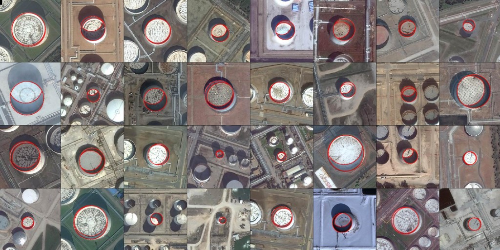
Oil tank identification - Copyright © Orbital Insight
Quant hedge funds have been doing this for a while now. What is more interesting is that with the increased availability of satellite imagery, deep learning libraries and cloud-based storage and processing, it is well within the capability of the determined quant trader to do something similar.
I will be writing tutorial articles in the future on how to carry out such analysis, which will hopefully allow you to develop and add some uncorrelated strategies to your own portfolio.
Software Libraries for Deep Learning
The popularity of deep learning means that there is no shortage of available open source software libraries. A full list can be found at Wikipedia here. The major contenders are Tensorflow, Torch, Theano and Caffe.
I don't want to dwell on the specifics of the pros and cons between these libraries. Ultimately they all help you build deep learning models, in varying programming languages/environments, with differing performance characteristics and APIs to do so. If you wish to investigate which one might be preferable for your own projects, it is best to follow the Wikipedia link above and compare.
I have picked Theano for these tutorials as it is Python based, has access to both the CPU as well as GPU and is a prerequisite for PyMC3, which some of you may have already installed for the article on Bayesian MCMC.
We'll now introduce Theano and eventually apply it to a simple logistic regression model.
Introduction to Theano
For this article series we will make use of the Python Theano library.
What is Theano?
Theano is a numerical computation library that allows you to define, optimise and evaluate mathematical expressions involving multi-dimensional arrays efficiently across the CPU or GPU[5].
What does this mean? Well, many machine learning models are built using large multi-dimensional arrays, which are often used to store parameter values or weights. In addition these models analyse data that is also stored in large multi-dimensional arrays. Thus it makes sense to use a library that can efficiently handle multi-dimensional data.
What makes Theano particularly attractive from a deep learning point of view is that it uses symbolic expressions. That is, rather than writing Python code directly for mathematical formulae, you utilise objects to represent the equation. Theano then takes this equation and figures out how best to run it in a manner completely transparent to the programmer. Of extreme importance for deep learning applications (especially those that utilise stochastic gradient descent) is the ability for expressions to be symbolically differentiated. We will discuss this fact in more detail below.
The key point is that Theano allows you to write model specifications rather than the model implementations. This is particularly useful as Theano is very well integrated into the GPU, which provides substantial speed-ups for deep learning training.
Hence Theano sits somewhere between NumPy and the Python symbolic mathematics library SymPy.
I should point out that it is not used solely for deep learning research. PyMC3, the Bayesian Probabilistic Programming library, is also partially written in Theano.
Theano Installation
The installation instructions for Theano are best followed from the actual site here as there are many variations of platforms and Python versions that are likely to be used.
I have had a few emails from individuals having difficulty installing PyMC3 under Anaconda. The reason was actually a problem installing Theano (which is a requirement for PyMC3). If you are trying to install Theano in Anaconda on Windows, then the following Stack Overflow post may be useful: How to install Theano on Anaconda Python 2.7 x64 on Windows?
This tutorial will certainly be easier to follow on a Unix-based system such as Linux/Ubuntu or Mac OS X. I believe it also makes it easier to interface with a GPU because I am unsure if a GPU can be accessed under Anaconda on Windows.
Now we will turn our attention to logistic regression and its implementation in Theano.
Logistic Regression with Theano
I've outlined above the case for why deep learning is something you should seriously consider taking a look at. In this section we're going to create our first statistical model - a multiclass logistic regression - using the Theano framework in order to understand how it all fits together. While this is not a deep learning technique per se it is an absolutely crucial first step towards understanding more complicated architectures such as multilayer perceptrons and convolution neural networks.
We're going to apply the logistic regression to a famous dataset known as the MNIST handwritten digit set. We'll show that we can achieve reasonable classification performance with this method. However the most important aspect is to show how to construct a non-trivial model in Theano and use this as a basis for more complex deep architecture models in future articles.
We'll proceed by firstly outlining what the MNIST dataset is. Then we will briefly discuss logistic regression. We will then explore stochastic gradient descent, which is an optimisation algorithm used to train models, including those within deep learning. We will then discuss likelihood functions in order to provide a "loss function" for training. Finally, we will build all of these techniques in Theano and then train/test the logistic regression model on the CPU and GPU.
In order to do this we will be closely following the DeepLearning.net tutorial on logistic regression. The code will be very similar. However I want to discuss it here in much more depth as I believe the level of understanding required in the original tutorial is a bit too advanced for many who might not have encountered numerical libraries such as Theano previously.
MNIST Dataset
The Mixed National Institute of Standards and Technology (MNIST) database[16] is a substantial set of handwritten digit images, which is frequently used for training and testing within the field of machine learning. It contains 60,000 training images and 10,000 testing images, all of which are 28x28 pixels in size.
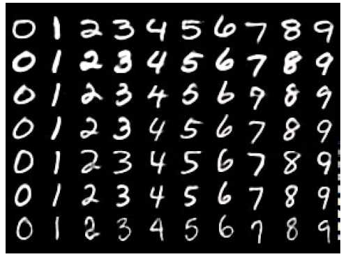
Examples of handwritten digits in the MNIST dataset.
Deep learning algorithms are currently at the state-of-the-art for classifiction performance on the MNIST dataset. In particular, a hierarchical convolution neural network approach achieved an error rate of just 0.23% in 2012.
We will be using the dataset throughout this article series as it is easy to work with and allows us to ascertain how the classification performance improves with increasing sophistication of the deep architectures we will study.
The MNIST dataset, in a form convenient to work with on these tutorials can be found here: http://www.iro.umontreal.ca/~lisa/deep/data/mnist/mnist.pkl.gz.
In order for this tutorial to be carried out correctly this file needs to be placed in the same directory as the following code, which I have named deep_logistic_regression_theano.py. It does not need to be decompressed. The decompression will be handled within Python via the gzip module.
In Linux/Ubuntu systems we can download the file directly through the command line:
$ wget http://www.iro.umontreal.ca/~lisa/deep/data/mnist/mnist.pkl.gz
Once again make sure to place this file in the same directory as the Python logistic regression file below.
Logistic Regression Model
In this tutorial we will make use of the probabilistic multiclass logistic regression model in order to classify the MNIST handwritten digits. Despite the name, logistic regression is actually a classification technique.
I will point out here that a detailed discussion of logistic regression is outside the scope of this article and would detract too much from the deep learning element! An introduction to the topic at an elementary mathematical level can be found in James et al[13], while a more advanced late undergraduate/early graduate discussion can be found in Hastie et al[12]. In addition I will be writing an article on the topic in the future and will post a link to it here once it is complete.
The idea of logistic regression in this example is to probabilisticly assign a class label to a digit image ("classify" it) once the logistic regression model has been "trained" on prior image-label pairs. Hence we are in a supervised learning regime.
If our class label response (the digit) is given by $Y$ and our input feature vector (the 28x28 pixel image) is given by $x$ then the probability of classification to a particular digit $k$ given a specific image $x$ is given by[12]:
\begin{eqnarray} P(Y=k \mid x) = \frac{\text{exp}(\beta_{k0} + \beta^{T}_k x)}{1 + \sum^{K-1}_{l=1} \text{exp}(\beta_{l0} + \beta^{T}_{l} x)} \end{eqnarray}
Where $k \in \{1,\ldots,K-1 \}$.
However we can rewrite this using matrices to simplify the list of parameters $\beta_j$. If we let $W$ be a matrix of weights and $b$ a vector bias (as in the original Theano Tutorial on Logistic Regression) then the probability becomes:
\begin{eqnarray} P(Y=k \mid x; W,b) = \frac{\text{exp}(W_k x + b_k}{\sum^{K}_{l=1} \text{exp}(W_l x + b_l)} \end{eqnarray}
At this stage, assuming we have some mechanism for finding the weight matrix $W$ and bias vector $b$, we can say that for a particular image feature vector $x$ that the most likely digit is given by $P(Y=k \mid x; W,b)$.
Thus we classify the image to a particular digit by taking the highest probability digit across all digits 0..9. Mathematically we write this using the $\text{argmax}$ function for the model prediction, $y_{\text{pred}}$:
\begin{eqnarray} y_{\text{pred}} = \text{argmax}_k P(Y=k \mid x; W,b) \end{eqnarray}
Thus it remains to (somehow) determine $W$ and $k$. This is where the concepts of loss functions, likelihoods and training come in. Prior to a discussion on likelihood we must discuss an optimisation algorithm called stochastic gradient descent that forms the basis for many future deep learning algorithms.
Stochastic Gradient Descent
An important part of deep learning algorithms is optimisation. Many deep learning architectures require minimising some form of objective function (or loss function) in order for a deep learning network to be "trained" or "learned".
A more familiar example is taken from classical statistics. For linear regression we may wish to use least squares in order to find the "line of best fit". Another example is given by the logistic regression used in this article. We need to optimise the negative log-likelihood (explained below) in order to ascertain the parameters of the logistic regression.
A particular optimisation method used frequently in deep learning is stochastic gradient descent. To describe how stochastic gradient descent works we first need to consider ordinary gradient descent.
Gradient descent is based on the idea that if we have an multivariable objective function or "optimisation surface" given by $f(x)$, with $f$ differentiable and $x \in \mathbb{R}^n$, then in a local region around a point $a$, $f$ decreases most rapidly if one moves in the direction of the negative gradient of $f$ at $a$. That is, we travel in the direction given by $- \nabla f(a)$. This basically says that the quickest way to get down a hill is to travel down the slope which is locally the steepest.
The algorithm is such that the next point reached, $x_{n+1}$, is equal to the previous point, $x_n$, minus the distance travelled in the direction of the steepest gradient:
\begin{eqnarray} x_{n+1} = x_n - \gamma_n \nabla f(x_n) \end{eqnarray}
Where $\gamma_n$ is a step-dependent parameter of how far to travel, known as the step size or learning rate.
The hope is that such a sequence of steps will converge to a desired local minimum. For the case of a deep learning network this should lead to a locally optimised "training", or "learning", parameter set.
In machine learning and other statistical estimation examples objective functions often have the form:
\begin{eqnarray} f(x) = \sum_{i=1}^n f_i (x) \end{eqnarray}
That is, the objective function is a sum of functions $f_i$, which are often associated with the $i$-th observation of the training/feature data set[14].
Stochastic gradient descent is similar to gradient descent except that instead of evaluating all partial derivatives of the summands $f_i$, $\frac{\partial f_i}{\partial x_j}$ at each step (which is computationally expensive) a random subset of partials is evaluated at every step. This leads to huge savings in computational cost, particularly for the high-dimensional deep learning networks we will be considering.
We will utilise stochastic gradient descent to evaluate our loss function below, as well as for all of the remaining articles on deep learning architectures.
The particular form of stochastic gradient descent utilised in this example is called minibatch stochastic gradient descent (MSGD) where more than one example of the training set is used per step. This has the effect of reducing the variance in the estimate of the gradient, as we are not so heavily dependent upon an individual training example for our gradient calculation. It also introduces an additional parameter, termed $B$, which is the size of the minibatch. We will discuss the size of $B$ for particular problems as they arise, since it does have an impact on convergence speed.
Negative Log-Likelihood Loss Function
As with advanced deep learning models classical statistics models require a mechanism that can generate the optimal parameters for prediction and inference. As we mentioned above a familiar example is the ordinary least squares approach for linear regression.
For logistic regression we need to use a concept known as maximum likelihood estimation (MLE). The basic idea with MLE is to estimate the parameters of a statistical model (such as the slope and intercept on a univariate linear regression) that "best" fit the data. In our case we are interested in selecting the best weight matrix $W$ and bias vector $b$ that fit our training data.
MLE works by selecting parameters that maximise the likelihood function. In this way it maximises the "agreement" of the model with the training data.
Many likelihood functions are in fact products of conditional probabilities. Since we are trying to maximise these likelihood functions we will need to take their partial derivatives with respect to the parameter values and set them to zero, as is usual for finding a maximum, minimum or stationary point in calculus.
Taking partial derivatives of products of probabilities leads to complex equations that become computationally expensive to evaluate at scale. Hence it is often easier to work with the logarithmic likelihood ("log-likelihood"). Taking a natural logarithm of a product reduces it to a sum of logarithms making differentiation far simpler. This works because the logarithm itself is a monotonic function meaning that the maximum of the log-likelihood is also the maximum of the likelihood. Hence we can use the log-likelihood in place of the likelihood function.
For logistic regression the negative log-likelihood for $N$ observations of training data is given by[12]:
\begin{eqnarray} \ell (\theta = \{ W, d \} \mid \mathcal{D}) = \sum_{i=1}^N \log (P(Y=k \mid x_i; \theta)) \end{eqnarray}
That is, the negative log likelihood of the parameters $\theta$ (which are the weight matrix $W$ and bias vector $b$) given the data $\mathcal{D}$ is equal to the sum across all training examples in $\mathcal{D}$ of the logarithm of the respective probabilities of a particular digit occuring given the particular $i$-th feature vector image, $x_i$, with the chosen parameters.
This is the loss function that we will be evaluating using Theano. Usually we would have to differentiate this function, which would lead to some complex expressions for its partial derivatives with respect to the parameters. In addition we would need to consider problems associated with numerical stability[15]. However we will see that we can use the Theano grad gradient operator to achieve this for us.
LogisticRegression Class in Theano
We're finally at a point where we can begin writing some Theano code. The full listing will be found later on in the file but I'd like to explain snippets as I go.
Before we begin we need to install Theano:
$ pip install theano
Once again, take a look at the Theano installation instructions for various platform installation guides.
As usual we'll start with the necessary library imports:
from __future__ import print_function

import gzip
import six.moves.cPickle as pickle
import timeit

import numpy as np
import theano
import theano.tensor as T
We're importing gzip and a faster version of pickle to decompress and deserialise the MNIST database. timeit is imported to calculate the wall-clock calculation time of the code for CPU/GPU comparison. Numpy is needed for the creation of the matrices and arrays, while we import the Theano tensor library as T for convenience.
Our first job is to create a class that encapsulates our logistic regression model. It will contain variables to store the weight matrix $W$ and the bias vector $b$. It will also contain a mechanism for calculating the probability of class membership $P(Y=k \mid x; W,b)$ and subsequently, a new class prediction $y_{\text{pred}}$.
Let's look at the code that will go into the initialisation of our LogisticRegression class. Our first snippet will define the weight matrix $W$:
self.W = theano.shared(
    value=np.zeros(
        (num_in, num_out), dtype=theano.config.floatX
    ),
    name='W', borrow=True
)
This snippet makes use of the theano.shared variable object, which allows us to share this symbolic variable between functions. It takes a shaped numpy matrix of zeros with a fixed type of floatX (we can set this to 32-bit or 64-bit). We have to give it a name, in this case 'W' and finally we use the borrow=True parameter in order to avoid costly deep copying. This is similar to passing by reference in C++. However this parameter will have no effect on a GPU. See here for a discussion on this. At this stage $W$ has NOT been "trained" and is just initialised to the zero matrix.
Now we create a similar snippet for the bias vector $b$. It is similar with the exception that we create a zero vector instead of a zero matrix:
self.b = theano.shared(
    value=np.zeros(
        (num_out,), dtype=theano.config.floatX
    ),
    name='b', borrow=True
)
we also need a a symbolic expression to store $P(Y=k \mid x; W,B)$. The code for this is given below:
self.p_y_x = T.nnet.softmax(T.dot(x, self.W) + self.b)
This looks rather complicated! So what's going on here? Firstly, you'll notice the inclusion of the softmax function. This is a particular mathematical function (which you can read about here) given by:
\begin{eqnarray} \sigma({\bf z}) = \frac{\text{exp}(z_k)}{\sum^{K}_{l=1} \text{exp}(z_l)} \end{eqnarray}
Where $k \in \{ 1, \ldots, K \}$. This is in fact the same form as our probability of class label $Y$ given feature vector $x$. Hence we can use the Theano implementation of the softmax function in our formulation. Notice that we're also using the dot operator between the vector $x$ and the weight matrix $W$, added to the bias vector $b$. Hence we have a symbolic representation of how to calculate our probability of class label.
The final variable to initialise is the mechanism for computing the actual class digit, given the probability. We saw above that this was characterised by the $\text{argmax}$ function. Hence you will likely find the following code snippet relatively easy to interpret as it simply makes use of the argmax function from Theano:
self.y_pred = T.argmax(self.p_y_x, axis=1)
This completes the initialisation of the class. Note once again that $W$ and $b$ have not been trained at this stage and are simply set to be zero tensors, that is tensors with all entries equal to zero.
Our next task is to use Theano operators to define the negative log-likelihood loss function in a symbolic manner so that we have a mechanism for evaluating the likelihood for any particular set of parameters $W$ and $b$. This would otherwise be complicated to express in code, if it were not for the operators provided by Theano:
def negative_log_likelihood(self, y):
    return -T.mean(T.log(self.p_y_x)[T.arange(y.shape[0]), y])
While the code is terse, there is a lot going on here and I want to explain it in depth. y.shape[0] is the number of examples in the minibatch of size $N$, which when plugged into T.arange(..) gives the symbolic vector containing the list of integers from $0$ to $N-1$.
The Theano log operator acts upon the probability of class $y$ given feature vector $x$ to produce a matrix of log probabilities. This matrix has many rows as there are training examples in the minibatch (i.e. $N$) and as many columns as there are classes/digits, $K$. In this case because we are considering the digits $0..9$, we have that $K=10$. Hence this matrix is an $N \times K$ = $N \times 10$ size matrix.
When these are combined T.log(self.p_y_x)[T.arange(y.shape[0]), y] provides us with a vector that contains the log likelihoods for each training example/class digit response pair. Hence this vector has length $N$. We take the mean (T.mean) of this vector to provide us with the average log likelihood across all training examples in the minibatch. Finally, we take the negative of it to give us the mean negative log likelihood across the training examples.
As you can see a reasonable amount of calculation is happening even within this one line. This is a major benefit of using Theano. It allows us to specify how to calculate an expression rather than force us to implement the calculation. We can leave the hard work of finding an optimal implementation to Theano.
The final task is to define a mechanism for calculating the error rate for a particular batch of digit predictions. To this end we define the errors method on the LogisticRegression class, which accepts a vector of digits y and compares it to the predicted vector self.y_pred:
def errors(self, y):
    # We first check whether the y vector has the same
    # dimension as the y prediction vector
    if y.ndim != self.y_pred.ndim:
        raise TypeError(
            "y should have the same shape as self.y_pred",
            ("y", y.type, "y_pred", self.y_pred.type)
        )
    # Check if y contains the correct (integer) types
    if y.dtype.startswith('int'):
        # We can use the Theano neq operator to return
        # vector of 1s or 0s, where 1 represents a
        # classification mistake
        return T.mean(T.neq(self.y_pred, y))
    else:
        raise NotImplementedError()
The method makes use of the Theano neq operator, which returns a vector of 1s or 0s, where 1 represents a classification mistake. This allows us to estimate the prediction accuracy in the training of the model below.
Training the Model
Before we can train the model it is necessary to decompress up the MNIST gzip file that we downloaded above, within Python.
In order to return the correct training, validation and test set feature-response pairs (i.e. image-digit pairs) we need a mechanism for creating Theano shared variables. This allows the data to be copied into GPU memory. If we were to copy a minibatch sequentially, it would degrade performance significantly as GPU memory transfer is slow. Here is the shared_dataset method that achieves this:
def shared_dataset(data_xy, borrow=True):
    """
    Create Theano shared variables to allow the data to
    be copied to the GPU to avoid performance-degrading
    sequential minibatch data copying.
    """
    data_x, data_y = data_xy
    shared_x = theano.shared(
        np.asarray(
            data_x, dtype=theano.config.floatX
        ), borrow=borrow
    )
    shared_y = theano.shared(
        np.asarray(
            data_y, dtype=theano.config.floatX
        ), borrow=borrow
    )
    return shared_x, T.cast(shared_y, 'int32')
The last line requires a little explanation. Since the GPU needs to store data in floating point format, and we require the digit values to be integers for training purposes, we cast the data to integer format.
The code to open up the gzipped MNIST data is as follows:
def load_mnist_data(filename):
    """
    Load the MNIST gzipped dataset into a
    test, validation and training set via
    the Python pickle library
    """
    # Use the gzip compression and pickle serialisation
    # libraries to open the MNIST images into training,
    # validation and testing sets
    with gzip.open(filename, 'rb') as gzf:
        try:
            train_set, valid_set, test_set = pickle.load(
                gzf, encoding='latin1'
            )
        except:
            train_set, valid_set, test_set = pickle.load(gzf)

    # Use the shared dataset function to create
    # Theano shared variables for GPU data copying
    test_set_x, test_set_y = shared_dataset(test_set)
    valid_set_x, valid_set_y = shared_dataset(valid_set)
    train_set_x, train_set_y = shared_dataset(train_set)

    # Create a list of tuples containing the
    # feature-response pairs for the training,
    # validation and test sets respectively
    rval = [
        (train_set_x, train_set_y),
        (valid_set_x, valid_set_y),
        (test_set_x, test_set_y)
    ]
    return rval
This is relatively straightforward. It uses a with context to open the file through the gzip library then deserialises the data via the Python pickle library, taking care with the encoding.
It then uses the shared_dataset function defined above to create Theano shared variables for the data (so it can be copied to the GPU in a performance-optimised manner). Finally, it returns a set of tuples of feature-response pairs for partition of the data into training, validation and testing sets.
Now that the code for loading the dataset has been outlined our attention turns to the stochastic gradient descent training method. This is a complex function and contains a lot of code. I will try and break it down into more manageable chunks. As we go through the article series we will see many examples of SGD training so don't be too concerned if you find this section a little tricky!
The first task is to define the function and its parameters:
def stoch_grad_desc_train_model(
    filename, gamma=0.13, epochs=1000, B=600
):
    """
    Train the logistic regression model using
    stochastic gradient descent.

    filename - File path of MNIST dataset
    gamma - Step size or "learning rate" for gradient descent
    epochs - Maximum number of epochs to run SGD
    B - The batch size for each minibatch
    """
    # Obtain the correct dataset partitions
    datasets = load_mnist_data(filename)
    train_set_x, train_set_y = datasets[0]
    valid_set_x, valid_set_y = datasets[1]
    test_set_x, test_set_y = datasets[2]

    # Calculate the number of minibatches for each of
    # the training, validation and test dataset partitions
    # Note the use of the // operator which is for
    # integer floor division, e.g.
    # 1.0//2 is equal to 0.0
    # 1//2 is equal to 0
    n_train_batches = train_set_x.get_value(borrow=True).shape[0] // B
    n_valid_batches = valid_set_x.get_value(borrow=True).shape[0] // B
    n_test_batches = test_set_x.get_value(borrow=True).shape[0] // B
The parameters of this function are the dataset filename, the step size (or learning rate) gamma, the maximum number of epochs to run the SGD algorithm for and the minibatch size B. The default values have been chosen based on those suggested by the original Theano logistic regression tutorial.
The function initially obtains the MNIST dataset and partitions it into training, validation and test sets. Subsequently the number of minibatches for each partition is calculated by dividing the sizes of each dataset by the batch size, $B$.
The next task is to build the logistic regression model:
    # BUILD THE MODEL
    # ===============
    print("Building the logistic regression model...")

    # Create symbolic variables for the minibatch data
    index = T.lscalar()  # Integer scalar value
    x = T.matrix('x')  # Feature vectors, i.e. the images
    y = T.ivector('y')  # Vector of integers representing digits

    # Instantiate the logistic regression model and assign the cost
    logreg = LogisticRegression(x=x, num_in=28**2, num_out=10)
    cost = logreg.negative_log_likelihood(y)  # This is what we minimise with SGD

    # Compiles a set of Theano functions for both the testing
    # and validation set that compute the errors on the model
    # in a particular minibatch
    test_model = theano.function(
        inputs=[index],
        outputs=logreg.errors(y),
        givens={
            x: test_set_x[index * B: (index + 1) * B],
            y: test_set_y[index * B: (index + 1) * B]
        }
    )

    validate_model = theano.function(
        inputs=[index],
        outputs=logreg.errors(y),
        givens={
            x: valid_set_x[index * B: (index + 1) * B],
            y: valid_set_y[index * B: (index + 1) * B]
        }
    )
Symbolic variables are created to store the minibatch data prior to the instantiation of the LogisticRegression class. Note the dimensionality of the inputs, which is 28x28 pixels for the MNIST handwriting images. The output dimensionality is 10, representing each of the digits from 0 to 9.
The next section creates a set of Theano functions, which compute the errors associated with a particular minibatch of testing and training data. They make use of the LogisticRegression errors method. Both of these compiled functions are used below.
The Theano symbolic grad operator is then used to calculate the gradient of the negative log-likelihood with respect to changes in the underlying parameters $W$ and $b$. At this point the stochastic gradient descent step is coded into the updates list. Finally a further compiled function is used, along with the updates=updates parameter to simultaneously evaluate the errors on the training minibatch but also perform the actual SGD update step on the parameters:
    # Use Theano to compute the symbolic gradients of the
    # cost function (negative log likelihood) with respect to
    # the underlying parameters W and b
    grad_W = T.grad(cost=cost, wrt=logreg.W)
    grad_b = T.grad(cost=cost, wrt=logreg.b)

    # This is the gradient descent step. It specifies a list of
    # tuple pairs, each of which contains a Theano variable and an
    # expression on how to update them on each step.
    updates = [
        (logreg.W, logreg.W - gamma * grad_W),
        (logreg.b, logreg.b - gamma * grad_b)
    ]

    # Similar to the above compiled Theano functions, except that
    # it is carried out on the training data AND updates the parameters
    # W, b as it evaluates the cost for the particular minibatch
    train_model = theano.function(
        inputs=[index],
        outputs=cost,
        updates=updates,
        givens={
            x: train_set_x[index * B: (index + 1) * B],
            y: train_set_y[index * B: (index + 1) * B]
        }
    )
The next part of the function concerns the actual training loop for the model:
    # TRAIN THE MODEL
    # ===============
    print("Training the logistic regression model...")

    # Set parameters to stop minibatch early
    # if performance is good enough
    patience = 5000  # Minimum number of examples to look at
    patience_increase = 2  # Increase by this for new best score
    improvement_threshold = 0.995  # Relative improvement threshold
    # Train through this number of minibatches before
    # checking performance on the validation set
    validation_frequency = min(n_train_batches, patience // 2)

    # Keep track of the validation loss and test scores
    best_validation_loss = np.inf
    test_score = 0.
    start_time = timeit.default_timer()
A variable called patience is defined. This is used to determine the initial minimum number of examples to look at in each minibatch. As the performance increases (i.e. the classification error decreases) this patience value is increased, as more samples per minibatch are needed in order to continuously increase the relative performance per minibatch.
A validation_frequency is also calculated to determine how often to assess the classification performance on the validation set. Finally we begin timing the training procedure through Python's timeit module.
The next section of the code concerns the main training loop. It is rather extensive. I will list the full code here and explain it in detail after the snippet:
    # Begin the training loop
    # The outer while loop loops over the number of epochs
    # The inner for loop loops over the minibatches
    finished = False
    cur_epoch = 0
    while (cur_epoch < epochs) and (not finished):
        cur_epoch = cur_epoch + 1
        # Minibatch loop
        for minibatch_index in range(n_train_batches):
            # Calculate the average likelihood for the minibatches
            minibatch_avg_cost = train_model(minibatch_index)
            iter = (cur_epoch - 1) * n_train_batches + minibatch_index

            if (iter + 1) % validation_frequency == 0:
                # If the current iteration has reached the validation
                # frequency then evaluate the validation loss on the
                # validation batches
                validation_losses = [
                    validate_model(i)
                    for i in range(n_valid_batches)
                ]
                this_validation_loss = np.mean(validation_losses)

                # Output current validation results
                print(
                    "Epoch %i, Minibatch %i/%i, Validation Error %f %%" % (
                        cur_epoch,
                        minibatch_index + 1,
                        n_train_batches,
                        this_validation_loss * 100.
                    )
                )

                # If we obtain the best validation score to date
                if this_validation_loss < best_validation_loss:
                    # If the improvement in the loss is within the
                    # improvement threshold, then increase the
                    # number of iterations ("patience") until the next check
                    if this_validation_loss < best_validation_loss *  \
                        improvement_threshold:
                        patience = max(patience, iter * patience_increase)
                    # Set the best loss to the new current (good) validation loss
                    best_validation_loss = this_validation_loss

                    # Now we calculate the losses on the minibatches
                    # in the test data set. Our "test_score" is the
                    # mean of these test losses
                    test_losses = [
                        test_model(i)
                        for i in range(n_test_batches)
                    ]
                    test_score = np.mean(test_losses)

                    # Output the current test results (indented)
                    print(
                        (
                            "     Epoch %i, Minibatch %i/%i, Test error of"
                            " best model %f %%"
                        ) % (
                            cur_epoch,
                            minibatch_index + 1,
                            n_train_batches,
                            test_score * 100.
                        )
                    )

                    # Serialise the model to disk using pickle
                    with open('best_model.pkl', 'wb') as f:
                        pickle.dump(logreg, f)
            # If the iterations exceed the current "patience"
            # then we are finished looping for this minibatch
            if iter > patience:
                done_looping = True
                break

    end_time = timeit.default_timer()
    print(
        (
            "Optimization complete with "
            "best validation score of %f %%,"
            "with test performance %f %%"
        ) % (best_validation_loss * 100., test_score * 100.)
    )
    print(
        'The code run for %d epochs, with %f epochs/sec' % (
            cur_epoch,
            1. * cur_epoch / (end_time - start_time)
        )
    )
    print("The code ran for %.1fs" % (end_time - start_time))
The outer while loop is a loop over the number of epochs. The inner loop is a for loop over the number of training minibatches. For each iteration of the inner loop, the average minibatch negative log-likelihood is calculated via the compiled train_model Theano function.
If the number of iterations reached is a multiple of the validation frequency the validation loss is calculation and output to the console. At this point a check is carried out to see if we have achieved the best validation loss to date. If so, then the "patience" is increased, requiring more iterations for subsequent validation improvement. At this point we also calculate the negative log-likelihood on the test set and output it to the console.
We then serialise (via pickle) the current "best" training model to disk. If we exceed the "patience" for this minibatch then we skip to the next minibatch. Finally we calculate the end time and output both the best validation loss and the total time to the console.
This completes the stochastic gradient descent of the logistic regression model with parameters $W$ and $b$.
Testing the Model
Compared to training the model the prediction of digits for new unseen test data is relatively simple. The following snippet shows how to carry out a prediction:
def test_model(filename, num_preds):
    """
    Test the model on unseen MNIST testing data
    """
    # Deserialise the best saved pickled model
    classifier = pickle.load(open('best_model.pkl'))

    # Use Theano to compile a prediction function
    predict_model = theano.function(
        inputs=[classifier.x],
        outputs=classifier.y_pred
    )

    # Load the MNIST dataset from "filename"
    # and isolate the testing data
    datasets = load_data(filename)
    test_set_x, test_set_y = datasets[2]
    test_set_x = test_set_x.get_value()

    # Predict the digits for num_preds images
    preds = predict_model(test_set_x[:num_preds])
    print(
        "Predicted digits for the first %s " \
        "images in test set:" % num_preds
    )
    print(preds)
If you've used the Scikit-Learn library for carrying out any supervised machine learning work you'll notiuce that the API is not too dissimilar.
The first task is to load the best_model.pkl pickled model and place it in the classifier variable. Subsequently we create a theano.function function, which takes as inputs the feature vector x and outputs the predicted digit values y_pred. Then we load the actual dataset and isolate the test set. Finally we create a vector of predictions, preds, that outputs the digit predictions for the first num_preds images in the test set.
Full Code
Tying all of the above functions and classes together produces the following code:
# deep_logistic_regression_theano.py

from __future__ import print_function

import gzip
import six.moves.cPickle as pickle
import timeit

import numpy as np
import theano
import theano.tensor as T


class LogisticRegression(object):
    def __init__(self, x, num_in, num_out):
        """
        LogisticRegression model specification in Theano.

        x - Feature vector
        num_in - Dimension of input image (28x28 = 784 for MNIST)
        num_out - Dimension of output (10 for digits 0..9)
        """
        # Initialise the shared weight matrix, 'W'
        self.W = theano.shared(
            value=np.zeros(
                (num_in, num_out), dtype=theano.config.floatX
            ),
            name='W', borrow=True
        )

        # Initialise the shared bias vector, 'b'
        self.b = theano.shared(
            value=np.zeros(
                (num_out,), dtype=theano.config.floatX
            ),
            name='b', borrow=True
        )

        # Symbolic expression for P(Y=k \mid x; \theta)
        self.p_y_x = T.nnet.softmax(T.dot(x, self.W) + self.b)

        # Symbolic expression for computing digit prediction
        self.y_pred = T.argmax(self.p_y_x, axis=1)

        # Model parameters
        self.params = [self.W, self.b]

        # Model feature data, x
        self.x = x

    def negative_log_likelihood(self, y):
        """
        Calculate the mean negative log likelihood across
        the N examples in the training data for a minibatch
        """
        return -T.mean(T.log(self.p_y_x)[T.arange(y.shape[0]), y])

    def errors(self, y):
        # We first check whether the y vector has the same
        # dimension as the y prediction vector
        if y.ndim != self.y_pred.ndim:
            raise TypeError(
                "y should have the same shape as self.y_pred",
                ("y", y.type, "y_pred", self.y_pred.type)
            )
        # Check if y contains the correct (integer) types
        if y.dtype.startswith('int'):
            # We can use the Theano neq operator to return
            # vector of 1s or 0s, where 1 represents a
            # classification mistake
            return T.mean(T.neq(self.y_pred, y))
        else:
            raise NotImplementedError()


def shared_dataset(data_xy, borrow=True):
    """
    Create Theano shared variables to allow the data to
    be copied to the GPU to avoid performance-degrading
    sequential minibatch data copying.
    """
    data_x, data_y = data_xy
    shared_x = theano.shared(
        np.asarray(
            data_x, dtype=theano.config.floatX
        ), borrow=borrow
    )
    shared_y = theano.shared(
        np.asarray(
            data_y, dtype=theano.config.floatX
        ), borrow=borrow
    )
    return shared_x, T.cast(shared_y, 'int32')


def load_mnist_data(filename):
    """
    Load the MNIST gzipped dataset into a
    test, validation and training set via
    the Python pickle library
    """
    # Use the gzip compression and pickle serialisation
    # libraries to open the MNIST images into training,
    # validation and testing sets
    with gzip.open(filename, 'rb') as gzf:
        try:
            train_set, valid_set, test_set = pickle.load(
                gzf, encoding='latin1'
            )
        except:
            train_set, valid_set, test_set = pickle.load(gzf)

    # Use the shared dataset function to create
    # Theano shared variables for GPU data copying
    test_set_x, test_set_y = shared_dataset(test_set)
    valid_set_x, valid_set_y = shared_dataset(valid_set)
    train_set_x, train_set_y = shared_dataset(train_set)

    # Create a list of tuples containing the
    # feature-response pairs for the training,
    # validation and test sets respectively
    rval = [
        (train_set_x, train_set_y),
        (valid_set_x, valid_set_y),
        (test_set_x, test_set_y)
    ]
    return rval


def stoch_grad_desc_train_model(
    filename, gamma=0.13, epochs=1000, B=600
):
    """
    Train the logistic regression model using
    stochastic gradient descent.

    filename - File path of MNIST dataset
    gamma - Step size or "learning rate" for gradient descent
    epochs - Maximum number of epochs to run SGD
    B - The batch size for each minibatch
    """
    # Obtain the correct dataset partitions
    datasets = load_mnist_data(filename)
    train_set_x, train_set_y = datasets[0]
    valid_set_x, valid_set_y = datasets[1]
    test_set_x, test_set_y = datasets[2]

    # Calculate the number of minibatches for each of
    # the training, validation and test dataset partitions
    # Note the use of the // operator which is for
    # integer floor division, e.g.
    # 1.0//2 is equal to 0.0
    # 1//2 is equal to 0
    n_train_batches = train_set_x.get_value(borrow=True).shape[0] // B
    n_valid_batches = valid_set_x.get_value(borrow=True).shape[0] // B
    n_test_batches = test_set_x.get_value(borrow=True).shape[0] // B

    # BUILD THE MODEL
    # ===============
    print("Building the logistic regression model...")

    # Create symbolic variables for the minibatch data
    index = T.lscalar()  # Integer scalar value
    x = T.matrix('x')  # Feature vectors, i.e. the images
    y = T.ivector('y')  # Vector of integers representing digits

    # Instantiate the logistic regression model and assign the cost
    logreg = LogisticRegression(x=x, num_in=28**2, num_out=10)
    cost = logreg.negative_log_likelihood(y)  # This is what we minimise with SGD

    # Compiles a set of Theano functions for both the testing
    # and validation set that compute the errors on the model
    # in a particular minibatch
    test_model = theano.function(
        inputs=[index],
        outputs=logreg.errors(y),
        givens={
            x: test_set_x[index * B: (index + 1) * B],
            y: test_set_y[index * B: (index + 1) * B]
        }
    )

    validate_model = theano.function(
        inputs=[index],
        outputs=logreg.errors(y),
        givens={
            x: valid_set_x[index * B: (index + 1) * B],
            y: valid_set_y[index * B: (index + 1) * B]
        }
    )

    # Use Theano to compute the symbolic gradients of the
    # cost function (negative log likelihood) with respect to
    # the underlying parameters W and b
    grad_W = T.grad(cost=cost, wrt=logreg.W)
    grad_b = T.grad(cost=cost, wrt=logreg.b)

    # This is the gradient descent step. It specifies a list of
    # tuple pairs, each of which contains a Theano variable and an
    # expression on how to update them on each step.
    updates = [
        (logreg.W, logreg.W - gamma * grad_W),
        (logreg.b, logreg.b - gamma * grad_b)
    ]

    # Similar to the above compiled Theano functions, except that
    # it is carried out on the training data AND updates the parameters
    # W, b as it evaluates the cost for the particular minibatch
    train_model = theano.function(
        inputs=[index],
        outputs=cost,
        updates=updates,
        givens={
            x: train_set_x[index * B: (index + 1) * B],
            y: train_set_y[index * B: (index + 1) * B]
        }
    )

    # TRAIN THE MODEL
    # ===============
    print("Training the logistic regression model...")

    # Set parameters to stop minibatch early
    # if performance is good enough
    patience = 5000  # Minimum number of examples to look at
    patience_increase = 2  # Increase by this for new best score
    improvement_threshold = 0.995  # Relative improvement threshold
    # Train through this number of minibatches before
    # checking performance on the validation set
    validation_frequency = min(n_train_batches, patience // 2)

    # Keep track of the validation loss and test scores
    best_validation_loss = np.inf
    test_score = 0.
    start_time = timeit.default_timer()

    # Begin the training loop
    # The outer while loop loops over the number of epochs
    # The inner for loop loops over the minibatches
    finished = False
    cur_epoch = 0
    while (cur_epoch < epochs) and (not finished):
        cur_epoch = cur_epoch + 1
        # Minibatch loop
        for minibatch_index in range(n_train_batches):
            # Calculate the average likelihood for the minibatches
            minibatch_avg_cost = train_model(minibatch_index)
            iter = (cur_epoch - 1) * n_train_batches + minibatch_index

            if (iter + 1) % validation_frequency == 0:
                # If the current iteration has reached the validation
                # frequency then evaluate the validation loss on the
                # validation batches
                validation_losses = [
                    validate_model(i)
                    for i in range(n_valid_batches)
                ]
                this_validation_loss = np.mean(validation_losses)

                # Output current validation results
                print(
                    "Epoch %i, Minibatch %i/%i, Validation Error %f %%" % (
                        cur_epoch,
                        minibatch_index + 1,
                        n_train_batches,
                        this_validation_loss * 100.
                    )
                )

                # If we obtain the best validation score to date
                if this_validation_loss < best_validation_loss:
                    # If the improvement in the loss is within the
                    # improvement threshold, then increase the
                    # number of iterations ("patience") until the next check
                    if this_validation_loss < best_validation_loss *  \
                        improvement_threshold:
                        patience = max(patience, iter * patience_increase)
                    # Set the best loss to the new current (good) validation loss
                    best_validation_loss = this_validation_loss

                    # Now we calculate the losses on the minibatches
                    # in the test data set. Our "test_score" is the
                    # mean of these test losses
                    test_losses = [
                        test_model(i)
                        for i in range(n_test_batches)
                    ]
                    test_score = np.mean(test_losses)

                    # Output the current test results (indented)
                    print(
                        (
                            "     Epoch %i, Minibatch %i/%i, Test error of"
                            " best model %f %%"
                        ) % (
                            cur_epoch,
                            minibatch_index + 1,
                            n_train_batches,
                            test_score * 100.
                        )
                    )

                    # Serialise the model to disk using pickle
                    with open('best_model.pkl', 'wb') as f:
                        pickle.dump(logreg, f)
            # If the iterations exceed the current "patience"
            # then we are finished looping for this minibatch
            if iter > patience:
                done_looping = True
                break

    end_time = timeit.default_timer()
    print(
        (
            "Optimization complete with "
            "best validation score of %f %%,"
            "with test performance %f %%"
        ) % (best_validation_loss * 100., test_score * 100.)
    )
    print(
        'The code run for %d epochs, with %f epochs/sec' % (
            cur_epoch,
            1. * cur_epoch / (end_time - start_time)
        )
    )
    print("The code ran for %.1fs" % (end_time - start_time))


def test_model(filename, num_preds):
    """
    Test the model on unseen MNIST testing data
    """
    # Deserialise the best saved pickled model
    classifier = pickle.load(open('best_model.pkl'))

    # Use Theano to compile a prediction function
    predict_model = theano.function(
        inputs=[classifier.x],
        outputs=classifier.y_pred
    )

    # Load the MNIST dataset from "filename"
    # and isolate the testing data
    datasets = load_mnist_data(filename)
    test_set_x, test_set_y = datasets[2]
    test_set_x = test_set_x.get_value()

    # Predict the digits for num_preds images
    preds = predict_model(test_set_x[:num_preds])
    print(
        "Predicted digits for the first %s " \
        "images in test set:" % num_preds
    )
    print(preds)


if __name__ == "__main__":
    # Specify the dataset and the number of
    # predictions to make on the testing data
    dataset_filename = "mnist.pkl.gz"
    num_preds = 20

    # Train the model via stochastic gradient descent
    stoch_grad_desc_train_model(dataset_filename)

    # Test the logistic regression on unseen test data
    test_model(dataset_filename, num_preds)
Running the Model on the CPU or GPU
To run the code on the CPU we can use the following command from the terminal. I've used the dollar symbol to indicate that this is a terminal command, so make sure not to include it when you copy and paste the code into the terminal:
$ THEANO_FLAGS=mode=FAST_RUN,device=cpu,floatX=float32 python deep_logistic_regression_theano.py
You should receive output similar to the following:
Building the logistic regression model...
Training the logistic regression model...
Epoch 1, Minibatch 83/83, Validation Error 12.458333 %
     Epoch 1, Minibatch 83/83, Test error of best model 12.375000 %
Epoch 2, Minibatch 83/83, Validation Error 11.010417 %
     Epoch 2, Minibatch 83/83, Test error of best model 10.958333 %
Epoch 3, Minibatch 83/83, Validation Error 10.312500 %
     Epoch 3, Minibatch 83/83, Test error of best model 10.312500 %
Epoch 4, Minibatch 83/83, Validation Error 9.875000 %
     Epoch 4, Minibatch 83/83, Test error of best model 9.833333 %
Epoch 5, Minibatch 83/83, Validation Error 9.562500 %
     Epoch 5, Minibatch 83/83, Test error of best model 9.479167 %
Epoch 6, Minibatch 83/83, Validation Error 9.322917 %
     Epoch 6, Minibatch 83/83, Test error of best model 9.291667 %
..
.. --TRUNCATED--
..
Epoch 71, Minibatch 83/83, Validation Error 7.520833 %
Epoch 72, Minibatch 83/83, Validation Error 7.510417 %
Epoch 73, Minibatch 83/83, Validation Error 7.500000 %
     Epoch 73, Minibatch 83/83, Test error of best model 7.489583 %
Epoch 74, Minibatch 83/83, Validation Error 7.479167 %
     Epoch 74, Minibatch 83/83, Test error of best model 7.489583 %
Optimization complete with best validation score of 7.479167 %,with test performance 7.489583 %
The code run for 1000 epochs, with 37.882747 epochs/sec
The code ran for 26.4s
Predicted digits for the first 20 images in test set:
[7 2 1 0 4 1 4 9 6 9 0 6 9 0 1 5 9 7 3 4]
On my desktop with an Intel Core i7-4770K, overclocked to 3.50Ghz, this took 26.4 seconds. Alternatively to run on the GPU enter the following command in the terminal:
$ THEANO_FLAGS=mode=FAST_RUN,device=gpu,floatX=float32 python deep_logistic_regression_theano.py
You should receive output similar to the following:
Using gpu device 0: GeForce GTX 780 Ti (CNMeM is disabled, cuDNN not available)
Building the logistic regression model...
Training the logistic regression model...
Epoch 1, Minibatch 83/83, Validation Error 12.458333 %
     Epoch 1, Minibatch 83/83, Test error of best model 12.375000 %
Epoch 2, Minibatch 83/83, Validation Error 11.010417 %
     Epoch 2, Minibatch 83/83, Test error of best model 10.958333 %
Epoch 3, Minibatch 83/83, Validation Error 10.312500 %
     Epoch 3, Minibatch 83/83, Test error of best model 10.312500 %
Epoch 4, Minibatch 83/83, Validation Error 9.875000 %
     Epoch 4, Minibatch 83/83, Test error of best model 9.833333 %
Epoch 5, Minibatch 83/83, Validation Error 9.562500 %
     Epoch 5, Minibatch 83/83, Test error of best model 9.479167 %
Epoch 6, Minibatch 83/83, Validation Error 9.322917 %
     Epoch 6, Minibatch 83/83, Test error of best model 9.291667 %
..
.. --TRUNCATED--
..
Epoch 71, Minibatch 83/83, Validation Error 7.520833 %
Epoch 72, Minibatch 83/83, Validation Error 7.510417 %
Epoch 73, Minibatch 83/83, Validation Error 7.500000 %
     Epoch 73, Minibatch 83/83, Test error of best model 7.489583 %
Epoch 74, Minibatch 83/83, Validation Error 7.479167 %
     Epoch 74, Minibatch 83/83, Test error of best model 7.489583 %
Optimization complete with best validation score of 7.479167 %,with test performance 7.489583 %
The code run for 1000 epochs, with 251.317223 epochs/sec
The code ran for 4.0s
Predicted digits for the first 20 images in test set:
[7 2 1 0 4 1 4 9 6 9 0 6 9 0 1 5 9 7 3 4]
On the same desktop machine with an NVidia CUDA-enabled GeForce GTX 780 Ti this took 4.0 seconds, which for this task is a speed-up factor of 6.6x. To put this in perspective a training task that takes a week on a CPU will only take just over a day on the GPU. Hence if you are serious about building a machine or cluster for deep learning research it is well worth considering the use of GPUs. They are simplest way to boost performance for most deep learning architectures.
Next Steps
While logistic regression is hardly a state of the art technique for classification purposes it does allow us to explore the Theano API, build a non-trivial model on a large dataset, train the model on both the CPU and GPU as well as predict new classifications from this model.
In the next article we are going to take a look at our first neural network model, namely the multilayer perceptron (MLP). We will build a MLP in Theano and use it, once again, for the same supervised classification task of predicting MNIST digits. We will see if we can improve the performance against our logistic regression model.
Additional Resources for Machine Learning, Deep Learning and GPUs
- Coursera: Machine Learning by Andrew Ng
- NVIDIA Self-Study Courses for Deep Learning
- Udacity: Intro to Parallel Programming - Using CUDA to Harness the Power of GPUs
- Tim Dettmers Blog - A Full Hardware Guide to Deep Learning
References
- [1] Very Brief Introduction to Machine Learning for AI, IFT6266 Winter 2010
- [2] Introduction to Deep Learning Algorithms, IFT6266 Winter 2010
- [3] Bengio, Y. (2009). Learning Deep Architectures for AI. Foundations and Trends in Machine Learning 2 (1), pg1-127
- [4] Deep Learning Tutorials, deeplearning.net
- [5] Bergstra, J. et al. (2010) "Theano: A CPU and GPU Math Expression Compiler". Proceedings of the Python for Scientific Computing Conference (SciPy) 2010. June 30 - July 3, Austin, TX
- [6] Nielson, M. (2015). "Neural Networks and Deep Learning", Determination Press
- [7] Playing Atari with Deep Reinforcement Learning, DeepMind Technologies
- [8] Silver, D. et al. (2016). Mastering the Game of Go with Deep Neural Networks and Tree Search, Nature 529, p484-489
- [9] Wikipedia: Deep Learning
- [10] Beissinger, M. (2013). "Deep Learning 101"
- [11] Längkvist, M.J. (2014). "A Review of Unsupervised Feature Learning and Deep Learning for Time-Series Modeling". Pattern Recognition Letters 42 (1)
- [12] Hastie, T., Tibshirani, R., Friedman, J. (2009) The Elements of Statistical Learning, Springer
- [13] James, G., Witten, D., Hastie, T., Tibshirani, R. (2013) An Introduction to Statistical Learning, Springer
- [14] Wikipedia: Stochastic Gradient Descent
- [15] Classifying MNIST digits using Logistic Regression, deeplearning.net
- [16] LeCun, Y., Cortes, C., Burges, C.J.C., (2012). MNIST Database of Handwritten Digits


