In this article we are going to consider a stastical machine learning method known as a Decision Tree. Decision Trees (DTs) are a supervised learning technique that predict values of responses by learning decision rules derived from features. They can be used in both a regression and a classification context. For this reason they are sometimes also referred to as Classification And Regression Trees (CART).
DT/CART models are an example of a more general area of machine learning known as adaptive basis function models. These models learn the features directly from the data, rather than being prespecified, as in some other basis expansions. However, unlike linear regression, these models are not linear in the parameters and so we are only able to compute a locally optimal maximum likelihood estimate (MLE) for the parameters[1].
DT/CART models work by partitioning the feature space into a number of simple rectangular regions, divided up by axis parallel splits. In order to obtain a prediction for a particular observation, the mean or mode of the training observations' responses, within the partition that the new observation belongs to, is used.
One of the primary benefits of using a DT/CART is that, by construction, it produces interpretable if-then-else decision rulesets, which are akin to graphical flowcharts.
Their main disadvantage lies in the fact that they are often uncompetitive with other supervised techniques such as support vector machines or deep neural networks in terms of prediction accuracy.
However they can become extremely competitive when used in an ensemble method such as with bootstrap aggregation ("bagging"), Random Forests or boosting.
In quantitative finance ensembles of DT/CART models are used in forecasting, either future asset prices/directions or liquidity of certain instruments. In future articles we will build trading strategies based off these methods.
Mathematical Overview
Under a probabilistic adaptive basis function specification the model $f({\bf x})$ is given by[1]:
\begin{eqnarray} f({\bf x}) = \mathbb{E}(y \mid {\bf x}) = \sum^{M}_{m=1} w_m \phi({\bf x}; {\bf v}_m) \end{eqnarray}
Where $w_m$ is the mean response in a particular region, $R_m$, and ${\bf v}_m$ represents how each variable is split at a particular threshold value. These splits define how the feature space in $R^p$ into $M$ separate "hyperblock" regions.
Decision Trees for Regression
Let us consider an abstract example of regression problem with two feature variables ($X_1$, $X_2$) and a numerical response $y$. This will allow us to easily visualise the nature of partitioning carried out by the tree.
In the following figure we can see a pre-grown tree for this particular example:
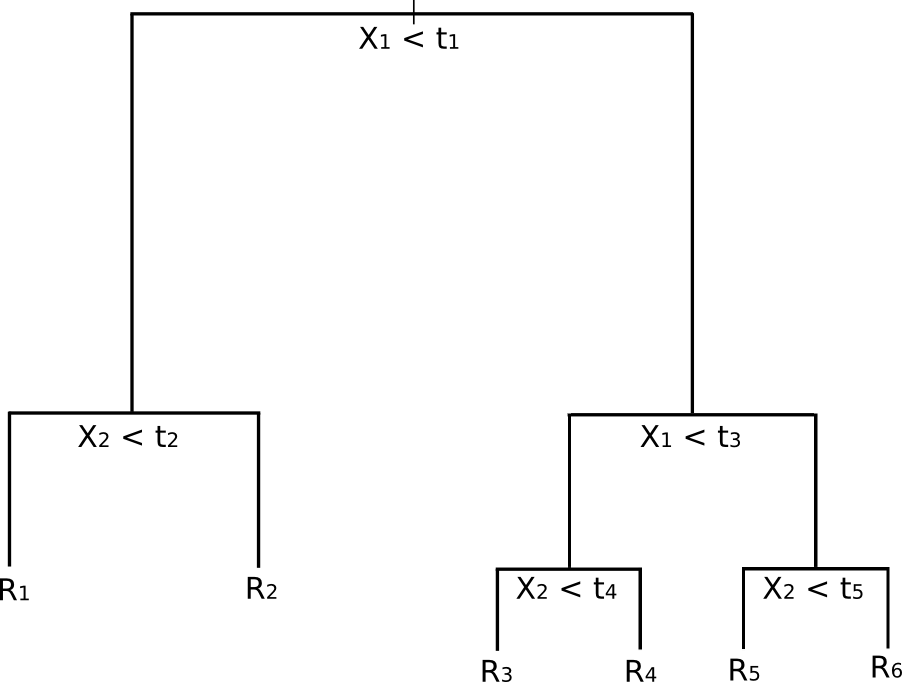
A Decision Tree with six separate regions
How does this correspond to a partitioning of the feature space? The following figure depicts a subset of $\mathbb{R}^2$ that contains our example data. Notice how the domain is partitioned using axis-parallel splits. That is, every split of the domain is aligned with one of the feature axes:
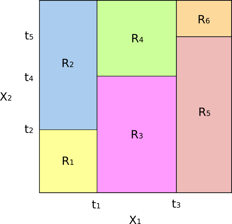
The resulting partition of the subset of $\mathbb{R}^2$ into six regional "blocks"
The concept of axis parallel splitting generalises straightforwardly to dimensions greater than two. For a feature space of size $p$, a subset of $\mathbb{R}^p$, the space is divided into $M$ regions, $R_m$, each of which is a $p$-dimensional "hyperblock".
We have yet to discuss how such a tree is "grown" or "trained". The following section outlines the algorithm for carrying this out.
Creating a Regression Tree and Making Predictions
The basic heuristic for creating a DT is as follows:
- Given $p$ features, partition the p-dimensional feature space (a subset of $\mathbb{R}^p$) into $M$ mutually distinct regions that fully cover the subset of feature space and do not overlap. These regions are given by $R_1,...,R_M$.
- Any new observation that falls into a particular partition $R_m$ has the estimated response given by the mean of all training observations with the partition, denoted by $w_m$.
However, this process doesn't actually describe how to form the partition in an algorithmic manner! For that we need to use a technique known as Recursive Binary Splitting (RBS)[2].
Recursive Binary Splitting
Our goal for this algorithm is to minimise some form of error criterion. In this particular instance we wish to minimise the Residual Sum of Squares (RSS), an error measure also used in linear regression settings. The RSS, in the case of a partitioned feature space with $M$ partitions is given by:
\begin{eqnarray} \text{RSS} = \sum^{M}_{m=1} \sum_{i \in R_m} ( y_i - \hat{y}_{R_m} )^2 \end{eqnarray}First we sum across all of the partitions of the feature space (the first summation sign) and then we sum across all test observations (indexed by $i$) in a particular partition (the second summation sign). We then take the squared difference of the response $y_i$ of a particular testing observation with the mean response $\hat{y}_{R_m}$ of the training observations within partition $m$.
Unfortunately it is too computationally expensive to consider all possible partitions of the feature space into $M$ rectangles (in fact the problem is NP-complete). Hence we must use a less computationally intensive, but more sophisticated search approach. This is where RBS comes in.
RBS approaches the problem by beginning at the top of the tree and splitting the tree into two branches, which creates a partition of two spaces. It carries out this particular split at the top of the tree multiple times and chooses the split of the features that minimises the (current) RSS.
At this point the tree creates a new branch in a particular partition and carries out the same procedure, that is, evaluates the RSS at each split of the partition and chooses the best.
This makes it a greedy algorithm, meaning that it carries out the evaluation for each iteration of the recursion, rather than "looking ahead" and continuing to branch before making the evaluations. It is this "greedy" nature of the algorithm that makes it computationally feasible and thus practical for use[1], [2].
At this stage we haven't outlined when this procedure actually terminates. There are a few criteria that we could consider, including limiting the maximum depth of the tree, ensuring sufficient training examples in each region and/or ensuring that the regions are sufficiently homogeneous such that the tree is relatively "balanced".
However, as with all supervised machine learning methods, we need to constantly be aware of overfitting. This motivates the concept of "pruning" the tree.
Pruning The Tree
Because of the ever-present worry of overfitting and the bias-variance tradeoff we need a means of adjusting the tree splitting process such that it can generalise well to test sets.
Since it is too costly to use cross-validation directly on every possible sub-tree combination while growing the tree, we need an alternative approach that still provides a good test error rate.
The usual approach is to grow the full tree to a prespecified depth and then carry out a procedure known as "pruning". One approach is called cost-complexity pruning and is described in detail in [2] and [3]. The basic idea is to introduce an additional tuning parameter, denoted by $\alpha$ that balances the depth of the tree and its goodness of fit to the training data. The approach used is similar to the LASSO technique developed by Tibshirani.
The details of the tree pruning will not concern us here as we can make use of Scikit-Learn to help us with this aspect.
Decision Trees for Classification
In this article we have concentrated almost exclusively on the regression case, but decision trees work equally well for classification, hence the "C" in CART models!
The only difference, as with all classification regimes, is that we are now predicting a categorical, rather than continuous, response value. In order to actually make a prediction for a categorical class we have to instead use the mode of the training region to which an observation belongs, rather than the mean value. That is, we take the most commonly occurring class value and assign it as the response of the observation.
In addition we need to consider alternative criteria for splitting the trees as the usual RSS score isn't applicable in the categorical setting. There are three that we will consider, which include the "hit rate", the Gini Index and Cross-Entropy[1], [2], [3].
Classification Error Rate/Hit Rate
Rather than seeing how far a numerical response is away from the mean value, as in the regression setting, we can instead define the "hit rate" as the fraction of training observations in a particular region that don't belong to the most widely occuring class. That is, the error is given by[1], [2]:
\begin{eqnarray} E = 1 - \text{argmax}_{c} (\hat{\pi}_{mc}) \end{eqnarray}
Where $\hat{\pi}_{mc}$ represents the fraction of training data in region $R_m$ that belong to class $c$.
Gini Index
The Gini Index is an alternative error metric that is designed to show how "pure" a region is. "Purity" in this case means how much of the training data in a particular region belongs to a single class. If a region $R_m$ contains data that is mostly from a single class $c$ then the Gini Index value will be small:
\begin{eqnarray} G = \sum_{c=1}^C \hat{\pi}_{mc} (1 - \hat{\pi}_{mc}) \end{eqnarray}
Cross-Entropy/Deviance
A third alternative, which is similar to the Gini Index, is known as the Cross-Entropy or Deviance:
\begin{eqnarray} D = - \sum_{c=1}^C \hat{\pi}_{mc} \text{log} \hat{\pi}_{mc} \end{eqnarray}
This motivates the question as to which error metric to use when growing a classification tree. I will state here that the Gini Index and Deviance are used more often than the Hit Rate, in order to maximise for prediction accuracy. We won't dwell on the reasons for this, but a good discussion can be found in the books provided in the References section below.
In future articles we will utilise the Scikit-Learn library to perform classification tasks and assess these error measures in order to determine how effective our predictions are on unseen data.
Advantages and Disadvantages of Decision Trees
As with all machine learning methods there are pros and cons to using DT/CARTs over other models:
Advantages
- DT/CART models are easy to interpret, as "if-else" rules
- The models can handle categorical and continuous features in the same data set
- The method of construction for DT/CART models means that feature variables are automatically selected, rather than having to use subset selection or similar
- The models are able to scale effectively on large datasets
Disadvantages
- Poor relative prediction performance compared to other ML models
- DT/CART models suffer from instability, which means they are very sensitive to small changes in the feature space. In the language of the bias-variance trade-off, they are high variance estimators.
While DT/CART models themselves suffer from poor prediction performance they are extremely competitive when utilised in an ensemble setting, via bootstrap aggregation ("bagging"), Random Forests or boosting.
In subsequent articles we will use the Decision Tree module of the Python scikit-learn library for classification and regression purposes on some quant finance datasets.
In addition we will show how ensembles of DT/CART models can perform extremely well for certain quant finance datasets.
Bibliographic Note
A gentle introduction to tree-based methods can be found in James et al (2013), which covers the basics of both DTs and their associated ensemble methods. A more rigourous account, pitched at the late undergraduate/early graduate mathematics/statistics level can be found in Hastie et al (2009). Murphy (2012) provides a discussion Adaptive Basis Function Models, of which DT/CART models are a subset. The book covers both the frequentist and Bayesian approach to these models. For the practitioner working on "real world" data (such as quants like us!), Kuhn et al (2013) is appropriate text pitched at a simpler level.
References
- [1] Murphy, K.P. (2012) Machine Learning A Probabilistic Perspective, MIT Press
- [2] James, G., Witten, D., Hastie, T., Tibshirani, R. (2013) An Introduction to Statistical Learning, Springer
- [3] Hastie, T., Tibshirani, R., Friedman, J. (2009) The Elements of Statistical Learning, Springer
- [4] Kuhn, M., Johnson, K. (2013) Applied Predictive Modeling, Springer


