In the previous article on cointegration in R we simulated two non-stationary time series that formed a cointegrated pair under a specific linear combination. We made use of the statistical Augmented Dickey-Fuller, Phillips-Perron and Phillips-Ouliaris tests for the presence of unit roots and cointegration.
A problem with the ADF test is that it does not provide us with the necessary $\beta$ regression parameter - the hedge ratio - for forming the linear combination of the two time series. In this article we are going to consider the Cointegrated Augmented Dickey-Fuller (CADF) procedure, which attempts to solve this problem. We've looked at CADF before using Python, but in this article we are going to implement our CADF function using R.
While CADF will help us identify the $\beta$ regression coefficient for our two series it will not tell us which of the two series is the dependent or independent variable for the regression. That is, the "response" value $Y$ from the "feature" $X$, in statistical machine learning parlance. We will show how to avoid this problem by calculating the test statistic in the ADF test and using it to determine which of the two regressions will correctly produce a stationary series.
Cointegrated Augmented Dickey Fuller Test
The main motivation for the CADF test is to determine an optimal hedging ratio to use between two pairs in a mean reversion trade, which was a problem that we identified with the analysis in the previous article. In essence it helps us determine how much of each pair to long and short when carrying out a pairs trade.
The CADF is a relatively simple procedure. We take a sample of historical data for two assets and then perform a linear regression between them, which produces $\alpha$ and $\beta$ regression coefficients, representing the intercept and slope, respectively. The slope term helps us identify how much of each pair to relatively trade.
Once the slope coefficient - the hedge ratio - has been obtained we can then perform an ADF test (as in the previous article) on the linear regression residuals in order to determine evidence of stationarity and hence cointegration.
We will use R to carry out the CADF procedure, making use of the tseries and quantmod libraries for the ADF test and historical data acquisition, respectively.
We will begin by constructing a synthetic data set, with known cointegrating properties, to see if the CADF procedure can recover the stationarity and hedging ratio. We will then apply the same analysis to some real historical future data, as a precursor to implementing some mean reversion trading strategies.
CADF on Simulated Data
We are now going to demonstrate the CADF approach on simulated data. We will use the same simulated time series from the previous article.
Recall that we artificially created two non-stationary time series that formed a stationary residual series under a specific linear combination.
We can use the R linear model lm function to carry out a linear regression between the two series. This will provide us with an estimate for the regression coefficients and thus the optimal hedge ratio between the two series.
We begin by importing the tseries library, necessary for the ADF test:
library("tseries")
Since we wish to use the same underlying stochastic trend series as in the previous article we set the seed for the random number generator as before:
set.seed(123)
In the previous article we created an underlying stochastic random walk time series, $z_t$:
z <- rep(0, 1000)
for (i in 2:1000) z[i] <- z[i-1] + rnorm(1)
We then created two subsequent series, which I will rename to $p_t$ and $q_t$ so that we do not confuse the original names $y_t$ and $x_t$ with the conventional names for regression reponses and predictors:
p <- q <- rep(0, 1000)
p <- 0.3*z + rnorm(1000)
q <- 0.6*z + rnorm(1000)
At this stage we can make use of the lm function, which calculates a linear regression between two vectors. In this instance we will set $q_t$ to be the independent variable and $p_t$ to be the dependent variable:
comb <- lm(p~q)
If we take a look at the comb linear regression model we can see that the estimate for the $\beta$ regression coefficient is approximately 0.5, which makes sense given that $q_t$ is twice dependent on $z_t$ compared to $p_t$ (0.6 compared to 0.3):
comb
The output is as follows:
Call:
lm(formula = p ~ q)

Coefficients:
(Intercept)            q
     0.1749       0.4745
Finally, we apply the ADF test to the residuals of the linear model in order to test for stationarity:
adf.test(comb$residuals, k=1)
The output is as follows:
  Augmented Dickey-Fuller Test

data:  comb$residuals
Dickey-Fuller = -23.4463, Lag order = 1, p-value = 0.01
alternative hypothesis: stationary

Warning message:
In adf.test(comb$residuals, k = 1) : p-value smaller than printed p-value
The Dickey-Fuller test statistic is very low, providing us with a low p-value. We can likely reject the null hypothesis of the presence of a unit root and conclude that we have a stationary series and hence a cointegrated pair. This is clearly not surprising given that we simulated the data to have these properties in the first place.
We are now going to apply the CADF procedure to multiple sets of historical financial data.
CADF on Financial Data
There are many ways of forming a cointegrating set of assets. A common source is to use ETFs that track similar characteristics. A good example is an ETF representing a basket of gold mining firms paired with an ETF that tracks the spot price of gold. Similarly for crude oil or any other commodity.
An alternative is to form tighter cointegrating pairs by considering separate share classes on the same stock, as with the Royal Dutch Shell example below. Another is the famous Berkshire Hathaway holding company, run by Warren Buffet and Charlie Munger, which also has A shares and B shares. However, in this instance we need to be careful because we must ask ourselves whether we would likely be able to form a profitable mean reversion trading strategy on such a pair, given how tight the cointegration is likely to be.
EWA and EWC
A famous example in the quant community of the CADF test applied to equities data is given by Ernie Chan[1]. He forms a cointegrating pair from two ETFs, with ticker symbols EWA and EWC, representing a set of Australian and Canadian equities baskets, respectively. The logic is that both of these countries are heavily commodities based and so will likely have a similar underlying stochastic trend.
Ernie makes uses of MatLab for his work, but this is an article about R. Hence I thought it would be instructive to utilise the same starting and ending dates for his historical analysis in order to see how the results compare.
The first task is to import the R quant finance library, quantmod, which will be helpful for us in downloading financial data:
library("quantmod")
We then need to obtain the backward-adjusted closing prices from Yahoo Finance for EWA and EWC across the exact period used in Ernie's work - April 26th 2006 to April 9th 2012:
getSymbols("EWA", from="2006-04-26", to="2012-04-09")
getSymbols("EWC", from="2006-04-26", to="2012-04-09")
We now place the adjusted prices into the ewaAdj and ewcAdj variables:
ewaAdj = unclass(EWA$EWA.Adjusted)
ewcAdj = unclass(EWC$EWC.Adjusted)
For completeness I will replicate the plots from Ernie's work, in order that you can see the same code in the R environment. Firstly, let's plot the adjusted ETF prices themselves.
To carry this out in R we need to utilise the par(new=T) command to append to a plot, rather than renew it. Notice that I've set the axes on both plot(...) commands to be equal and have not added axes to the second plot. If we don't do this the plot becomes cluttered and illegible:
plot(ewaAdj, type="l", xlim=c(0, 1500), ylim=c(5.0, 35.0), xlab="April 26th 2006 to April 9th 2012", ylab="ETF Backward-Adjusted Price in USD", col="blue")
par(new=T)
plot(ewcAdj, type="l", xlim=c(0, 1500), ylim=c(5.0, 35.0), axes=F, xlab="", ylab="", col="red")
par(new=F)
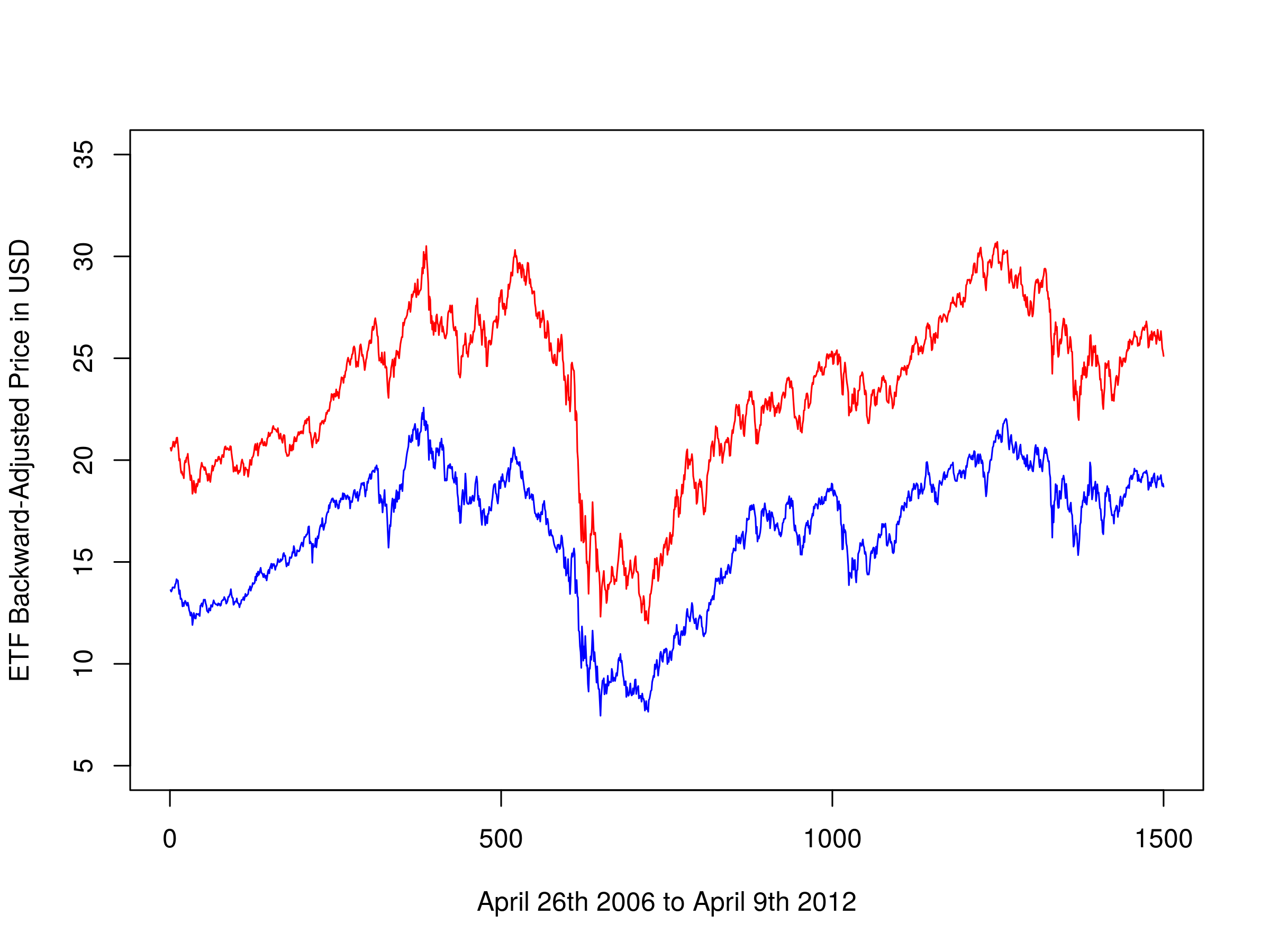 Backward-adjusted closing prices of EWA and EWC
You will notice that it differs slightly from the chart given in Ernie's work as we are plotting the adjusted prices here, rather than the unadjusted closing prices. We can also create a scatter plot of their prices:
plot(ewaAdj, ewcAdj, xlab="EWA Backward-Adjusted Prices", ylab="EWC Backward-Adjusted Prices")
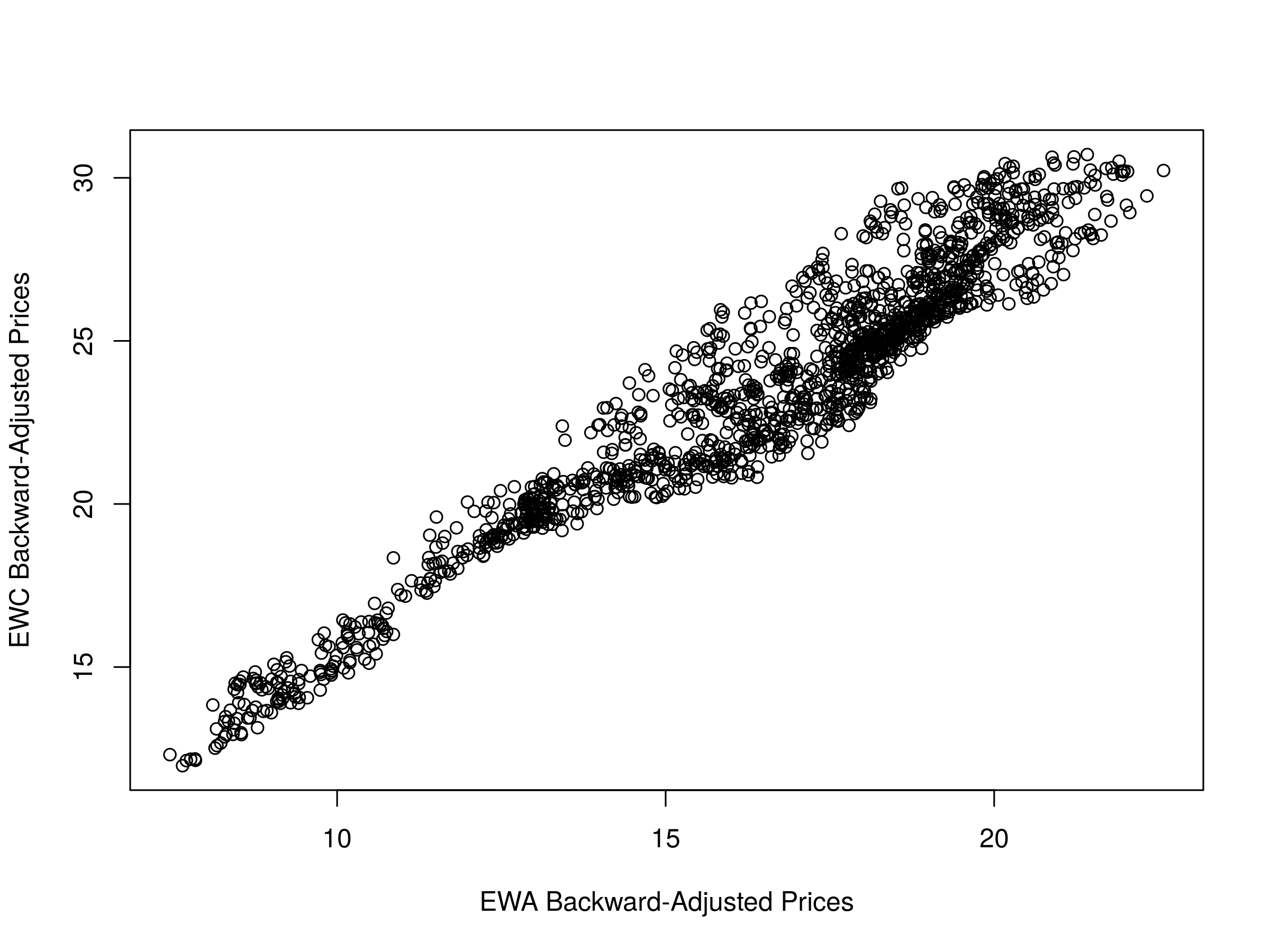 Scatter plot of backward-adjusted closing prices for EWA and EWC
At this stage we need to perform the linear regressions between the two price series. However, we have previously mentioned that it is unclear as to which series is the dependent variable and which is the independent variable for the regression. Thus we will try both and make a choice based on the negativity of the ADF test statistic. We will use the R linear model (lm) function for the regression:
comb1 = lm(ewcAdj~ewaAdj)
comb2 = lm(ewaAdj~ewcAdj)
This will provide us with the intercept and regression coefficient for these pairs. We can plot the residuals and visually assess the stationarity of the series:
plot(comb1$residuals, type="l", xlab="April 26th 2006 to April 9th 2012", ylab="Residuals of EWA and EWC regression")
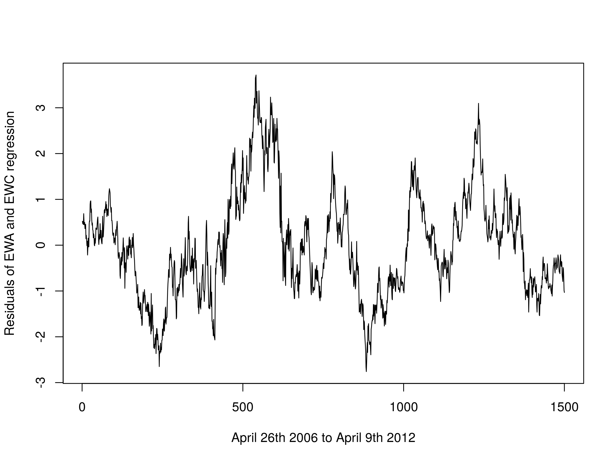 Residuals of the first linear combination of EWA and EWC
We can also view the regression coefficients starting with EWA as the independent variable:
comb1
The output is as follows:
Call:
lm(formula = ewcAdj ~ ewaAdj)

Coefficients:
(Intercept)       ewaAdj
      3.809        1.194
This provides us with an intercept of $\alpha=3.809$ and a $\beta=1.194$. Similarly for EWC as the independent variable:
comb2
The output is as follows:
Call:
lm(formula = ewaAdj ~ ewcAdj)

Coefficients:
(Intercept)       ewcAdj
     -1.638        0.771
This provides us with an intercept $\alpha=-1.638$ and a $\beta=0.771$. The key issue here is that they are not equal to the previous regression coefficients. Hence we must use the ADF test statistic in order to determine the optimal hedge ratio. For EWA as the independent variable:
adf.test(comb1$residuals, k=1)
The output is as follows:
    Augmented Dickey-Fuller Test

data:  comb1$residuals
Dickey-Fuller = -3.6357, Lag order = 1, p-value = 0.02924
alternative hypothesis: stationary
Our test statistic gives a p-value less than 0.05 providing evidence that we can reject the null hypothesis of a unit root at the 5% level. Similarly for EWC as the independent variable:
adf.test(comb2$residuals, k=1)
The output is as follows:
    Augmented Dickey-Fuller Test

data:  comb2$residuals
Dickey-Fuller = -3.6457, Lag order = 1, p-value = 0.02828
alternative hypothesis: stationary
Once again we have evidence to reject the null hypothesis of the presence of a unit root, leading to evidence for a stationary series (and cointegrated pair) at the 5% level.
The ADF test statistic for EWC as the independent variable is smaller (more negative) than that for EWA as the independent variable and hence we will choose this as our linear combination for any future trading implementations.
RDS-A and RDS-B
A common method of obtaining a strong cointegrated relationship is to take two publicly traded share classes of the same underlying equity. One such pair is given by the London-listed Royal Dutch Shell oil major, with its two share classes RDS-A and RDS-B.
We can replicate the above steps for RDS-A and RDS-B as we did for EWA and EWC. The full code to carry this out is given below. The only minor difference is that we need to utilise the get("...") R function, since quantmod pulls in RDS-A as the variable "RDS-A". R does not like hyphens in variable names as the minus operator takes precedence. Hence we need to use get as a workaround:
getSymbols("RDS-A", from="2006-01-01", to="2015-12-31")
getSymbols("RDS-B", from="2006-01-01", to="2015-12-31")
RDSA <- get("RDS-A")
RDSB <- get("RDS-B")
rdsaAdj = unclass(RDSA$"RDS-A.Adjusted")
rdsbAdj = unclass(RDSB$"RDS-B.Adjusted")
We can plot both share classes on the same chart. Clearly they are tightly cointegrated:
plot(rdsaAdj, type="l", xlim=c(0, 2517), ylim=c(25.0, 80.0), xlab="January 1st 2006 to December 31st 2015", ylab="RDS-A and RDS-B Backward-Adjusted Closing Price in GBP", col="blue")
par(new=T)
plot(rdsbAdj, type="l", xlim=c(0, 2517), ylim=c(25.0, 80.0), axes=F, xlab="", ylab="", col="red")
par(new=F)
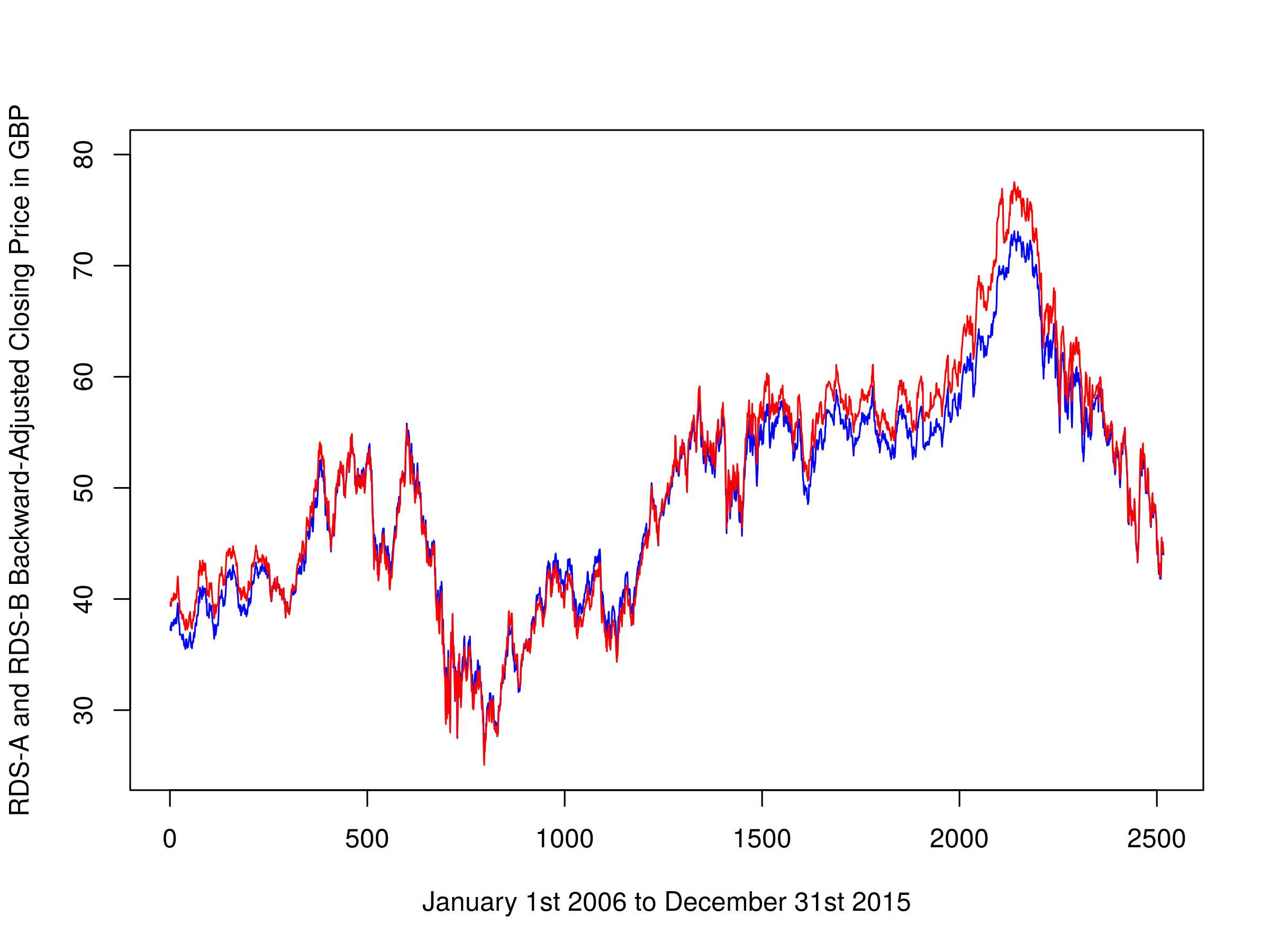 Backward-adjusted closing prices of RDS-A and RDS-B
We can also plot a scatter graph of the two price series. It is apparent how tight the linear relationship between them is. This is no surprise given that they track the same underlying equity:
plot(rdsaAdj, rdsbAdj, xlab="RDS-A Backward-Adjusted Prices", ylab="RDS-B Backward-Adjusted Prices")
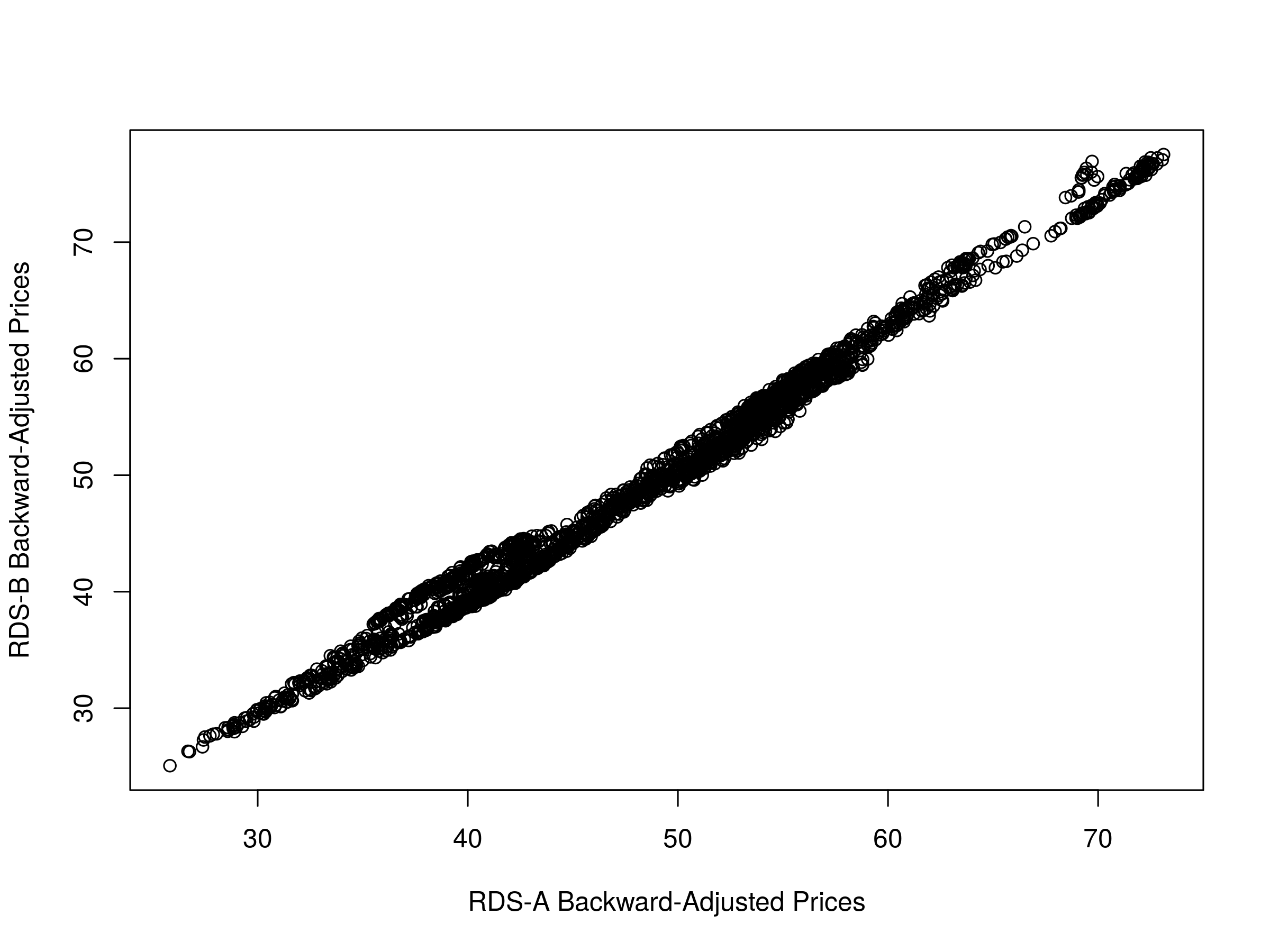 Scatter plot of backward-adjusted closing prices for RDS-A and RDS-B
Once again we utilise the linear model lm function to ascertain the regression coefficients, making sure to swap the dependent and independent variables for the second regression. We can then plot the residuals of the first regression:
comb1 = lm(rdsaAdj~rdsbAdj)
comb2 = lm(rdsbAdj~rdsaAdj)
plot(comb1$residuals, type="l", xlab="January 1st 2006 to December 31st 2015", ylab="Residuals of RDS-A and RDS-B regression")
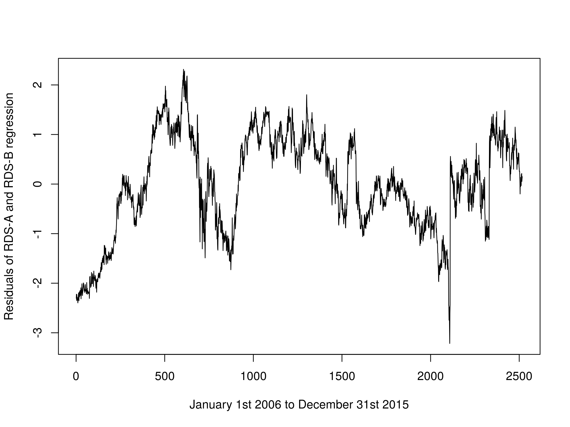 Residuals of the first linear combination of RDS-A and RDS-B
Finally, we can calculate the ADF test-statistic to ascertain the optimal hedge ratio. For the first linear combination:
adf.test(comb1$residuals, k=1)
The output is as follows:
  Augmented Dickey-Fuller Test

data:  comb1$residuals
Dickey-Fuller = -4.0537, Lag order = 1, p-value = 0.01
alternative hypothesis: stationary

Warning message:
In adf.test(comb1$residuals, k = 1) : p-value smaller than printed p-value
And for the second:
adf.test(comb2$residuals, k=1)
The output is as follows:
  Augmented Dickey-Fuller Test

data:  comb2$residuals
Dickey-Fuller = -3.9846, Lag order = 1, p-value = 0.01
alternative hypothesis: stationary

Warning message:
In adf.test(comb2$residuals, k = 1) : p-value smaller than printed p-value
Since the first linear combination has the smallest Dickey-Fuller statistic, we conclude that this is the optimal linear regression. In any subsequent trading strategy we would utilise these regression coefficients for our relative long-short positioning.
Next Steps
We have utilised the CADF to obtain the optimal hedge ratio for two cointegrated time series. In subsequent articles we will consider the Johansen test, which will allow us to form cointegrating time series for more than two assets, providing a much larger trading universe from which to pick strategies.
In addition we will consider the fact that the hedge ratio itself is not stationary and as such will utilise techniques to update our hedge ratio as new information arrives. We can utilise the Bayesian approach of the Kalman Filter for this.
Once we have examined these tests we will apply them to a set of trading strategies built in QSTrader and see how they perform with realistic transaction costs.
References
- [1] Chan, E. P. (2013) Algorithmic Trading: Winning Strategies and their Rationale, Wiley
- [2] Turan, D. (2013) Cointegration Tests (ADF and Johansen) within R
Full Code
library("quantmod")
library("tseries")

## Set the random seed to 123
set.seed(123)

## SIMULATED DATA

## Create a simulated random walk
z <- rep(0, 1000)
for (i in 2:1000) z[i] <- z[i-1] + rnorm(1)

## Create two non-stationary series based on the
## simulated random walk
p <- q <- rep(0, 1000)
p <- 0.3*z + rnorm(1000)
q <- 0.6*z + rnorm(1000)

## Perform a linear regression against the two
## simulated series in order to assess the hedge ratio
comb <- lm(p~q)

## FINANCIAL DATA - EWA/EWC

## Obtain EWA and EWC for dates corresponding to Chan (2013)
getSymbols("EWA", from="2006-04-26", to="2012-04-09")
getSymbols("EWC", from="2006-04-26", to="2012-04-09")

## Utilise the backwards-adjusted closing prices
ewaAdj = unclass(EWA$EWA.Adjusted)
ewcAdj = unclass(EWC$EWC.Adjusted)

## Plot the ETF backward-adjusted closing prices
plot(ewaAdj, type="l", xlim=c(0, 1500), ylim=c(5.0, 35.0), xlab="April 26th 2006 to April 9th 2012", ylab="ETF Backward-Adjusted Price in USD", col="blue")
par(new=T)
plot(ewcAdj, type="l", xlim=c(0, 1500), ylim=c(5.0, 35.0), axes=F, xlab="", ylab="", col="red")
par(new=F)

## Plot a scatter graph of the ETF adjusted prices
plot(ewaAdj, ewcAdj, xlab="EWA Backward-Adjusted Prices", ylab="EWC Backward-Adjusted Prices")

## Carry out linear regressions twice, swapping the dependent
## and independent variables each time, with zero drift
comb1 = lm(ewcAdj~ewaAdj)
comb2 = lm(ewaAdj~ewcAdj)

## Plot the residuals of the first linear combination
plot(comb1$residuals, type="l", xlab="April 26th 2006 to April 9th 2012", ylab="Residuals of EWA and EWC regression")

## Now we perform the ADF test on the residuals,
## or "spread" of each model, using a single lag order
adf.test(comb1$residuals, k=1)
adf.test(comb2$residuals, k=1)

## FINANCIAL DATA - RDS-A/RDS-B

## Obtain RDS equities prices for a recent ten year period
getSymbols("RDS-A", from="2006-01-01", to="2015-12-31")
getSymbols("RDS-B", from="2006-01-01", to="2015-12-31")

## Avoid the hyphen in the name of each variable
RDSA <- get("RDS-A")
RDSB <- get("RDS-B")

## Utilise the backwards-adjusted closing prices
rdsaAdj = unclass(RDSA$"RDS-A.Adjusted")
rdsbAdj = unclass(RDSB$"RDS-B.Adjusted")

## Plot the ETF backward-adjusted closing prices
plot(rdsaAdj, type="l", xlim=c(0, 2517), ylim=c(25.0, 80.0), xlab="January 1st 2006 to December 31st 2015", ylab="RDS-A and RDS-B Backward-Adjusted Closing Price in GBP", col="blue")
par(new=T)
plot(rdsbAdj, type="l", xlim=c(0, 2517), ylim=c(25.0, 80.0), axes=F, xlab="", ylab="", col="red")
par(new=F)

## Plot a scatter graph of the
## Royal Dutch Shell adjusted prices
plot(rdsaAdj, rdsbAdj, xlab="RDS-A Backward-Adjusted Prices", ylab="RDS-B Backward-Adjusted Prices")

## Carry out linear regressions twice, swapping the dependent
## and independent variables each time, with zero drift
comb1 = lm(rdsaAdj~rdsbAdj)
comb2 = lm(rdsbAdj~rdsaAdj)

## Plot the residuals of the first linear combination
plot(comb1$residuals, type="l", xlab="January 1st 2006 to December 31st 2015", ylab="Residuals of RDS-A and RDS-B regression")

## Now we perform the ADF test on the residuals,
## or "spread" of each model, using a single lag order
adf.test(comb1$residuals, k=1)
adf.test(comb2$residuals, k=1)


