Updated for Python 3.8, April 2022
In the previous article on Bayesian statistics we examined Bayes' rule and considered how it allowed us to rationally update beliefs about uncertainty as new evidence came to light. We mentioned briefly that such techniques are becoming extremely important in the fields of data science and quantitative finance.
In this article we are going to expand on the coin-flip example that we studied in the previous article by discussing the notion of Bernoulli trials, the beta distribution and conjugate priors.
Our goal in this article is to allow us to carry out what is known as "inference on a binomial proportion". That is, we will be studying probabilistic situations with two outcomes (e.g. a coin-flip) and trying to estimate the proportion of a repeated set of events that come up heads or tails.
Our goal is to estimate how fair a coin is. We will use that estimate to make predictions about how many times it will come up heads when we flip it in the future.
While this may sound like a rather academic example, it is actually substantially more applicable to real-world applications than may first appear. Consider the following scenarios:
- Engineering: Estimating the proportion of aircraft turbine blades that possess a structural defect after fabrication
- Social Science: Estimating the proportion of individuals who would respond "yes" on a census question
- Medical Science: Estimating the proportion of patients who make a full recovery after taking an experimental drug to cure a disease
- Corporate Finance: Estimating the proportion of transactions in error when carrying out financial audits
- Data Science: Estimating the proportion of individuals who click on an ad when visiting a website
As can be seen, inference on a binomial proportion is an extremely important statistical technique and will form the basis of many of the articles on Bayesian statistics that follow.
The Bayesian Approach
While we motivated the concept of Bayesian statistics in the previous article, I want to outline first how our analysis will proceed. This will motivate the following (rather mathematically heavy) sections and give you a "bird's eye view" of what a Bayesian approach is all about.
As we stated above, our goal is estimate the fairness of a coin. Once we have an estimate for the fairness, we can use this to predict the number of future coin flips that will come up heads.
We will learn about the specific techniques as we go while we cover the following steps:
- Assumptions - We will assume that the coin has two outcomes (i.e. it won't land on its side), the flips will appear randomly and will be completely independent of each other. The fairness of the coin will also be stationary, that is it won't alter over time. We will denote the fairness by the parameter $\theta$.
- Prior Beliefs - To carry out a Bayesian analysis, we must quantify our prior beliefs about the fairness of the coin. This comes down to specifying a probability distribution on our beliefs of this fairness. We will use a relatively flexible probability distribution called the beta distribution to model our beliefs.
- Experimental Data - We will carry out some (virtual) coin-flips in order to give us some hard data. We will count the number of heads $z$ that appear in $N$ flips of the coin. We will also need a way of determining the probability of such results appearing, given a particular fairness, $\theta$, of the coin. For this we will need to discuss likelihood functions, and in particular the Bernoulli likelihood function.
- Posterior Beliefs - Once we have a prior belief and a likelihood function, we can use Bayes' rule in order to calculate a posterior belief about the fairness of the coin. We couple our prior beliefs with the data we have observed and update our beliefs accordingly. Luckily for us, if we use a beta distribution as our prior and a Bernoulli likelihood we also get a beta distribution as a posterior. These are known as conjugate priors.
- Inference - Once we have a posterior belief we can estimate the coin's fariness $\theta$, predict the probability of heads on the next flip or even see how the results depend upon different choices of prior beliefs. The latter is known as model comparison.
At each step of the way we will be making visualisations of each of these functions and distributions using the Seaborn plotting package for Python. Seaborn sits "on top" of Matplotlib, but has far better defaults for statistical plotting. For some interesting examples of what Seaborn can do, take a look at the gallery.
Assumptions of the Approach
As with all models we need to make some assumptions about our situation.
- We are going to assume that our coin can only have two outcomes, that is it can only land on its head or tail and never on its side
- Each flip of the coin is completely independent of the others, i.e. we have independent and identically distributed (i.i.d.) coin flips
- The fairness of the coin does not change in time, that is it is stationary
With these assumptions in mind, we can now begin discussing the Bayesian procedure.
Recalling Bayes' Rule
In the previous article we outlined Bayes' rule. I've repeated the box callout here for completeness:
Bayes' Rule for Bayesian Inference
\begin{eqnarray} P(\theta|D) = P(D|\theta) \; P(\theta) \; / \; P(D) \end{eqnarray}Where:
- $P(\theta)$ is the prior. This is the strength in our belief of $\theta$ without considering the evidence $D$. Our prior view on the probability of how fair the coin is.
- $P(\theta|D)$ is the posterior. This is the (refined) strength of our belief of $\theta$ once the evidence $D$ has been taken into account. After seeing 4 heads out of 8 flips, say, this is our updated view on the fairness of the coin.
- $P(D|\theta)$ is the likelihood. This is the probability of seeing the data $D$ as generated by a model with parameter $\theta$. If we knew the coin was fair, this tells us the probability of seeing a number of heads in a particular number of flips.
- $P(D)$ is the evidence. This is the probability of the data as determined by summing (or integrating) across all possible values of $\theta$, weighted by how strongly we believe in those particular values of $\theta$. If we had multiple views of what the fairness of the coin is (but didn't know for sure), then this tells us the probability of seeing a certain sequence of flips for all possibilities of our belief in the coin's fairness.
Note that we have three separate components to specify, in order to calcute the posterior. They are the likelihood, the prior and the evidence. In the following sections we are going to discuss exactly how to specify each of these components for our particular case of inference on a binomial proportion.
The Likelihood Function
We have just outlined Bayes' rule and have seen that we must specify a likelihood function, a prior belief and the evidence (i.e. a normalising constant). In this section we are going to consider the first of these components, namely the likelihood.
Bernoulli Distribution
Our example is that of a sequence of coin flips. We are interested in the probability of the coin coming up heads. In particular, we are interested in the probability of the coin coming up heads as a function of the underlying fairness parameter $\theta$.
This will take a functional form, $f$. If we denote by $k$ the random variable that describes the result of the coin toss, which is drawn from the set $\{1,0\}$, where $k=1$ represents a head and $k=0$ represents a tail, then the probability of seeing a head, with a particular fairness of the coin, is given by:
\begin{eqnarray} P(k = 1 | \theta) = f(\theta) \end{eqnarray}We can choose a particularly succint form for $f(\theta)$ by simply stating the probability is given by $\theta$ itself, i.e. $f(\theta) = \theta$. This leads to the probability of a coin coming up heads to be given by:
\begin{eqnarray} P(k = 1 | \theta) = \theta \end{eqnarray}And the probability of coming up tails as:
\begin{eqnarray} P(k = 0 | \theta) = 1-\theta \end{eqnarray}This can also be written as:
\begin{eqnarray} P(k | \theta) = \theta^k (1 - \theta)^{1-k} \end{eqnarray}Where $k \in \{1, 0\}$ and $\theta \in [0,1]$.
This is known as the Bernoulli distribution. It gives the probability over two separate, discrete values of $k$ for a fixed fairness parameter $\theta$.
In essence it tells us the probability of a coin coming up heads or tails depending on how fair the coin is.
Bernoulli Likelihood Function
We can also consider another way of looking at the above function. If we consider a fixed observation, i.e. a known coin flip outcome, $k$, and the fairness parameter $\theta$ as a continuous variable then:
\begin{eqnarray} P(k | \theta) = \theta^k (1 - \theta)^{1-k} \end{eqnarray}tells us the probability of a fixed outcome $k$ given some particular value of $\theta$. As we adjust $\theta$ (e.g. change the fairness of the coin), we will start to see different probabilities for $k$.
This is known as the likelihood function of $\theta$. It is a function of a continuous $\theta$ and differs from the Bernoulli distribution because the latter is actually a discrete probability distribution over two potential outcomes of the coin-flip $k$.
Note that the likelihood function is not actually a probability distribution in the true sense since integrating it across all values of the fairness parameter $\theta$ does not actually equal 1, as is required for a probability distribution.
We say that $P(k | \theta) = \theta^k (1 - \theta)^{1-k}$ is the Bernoulli likelihood function for $\theta$.
Multiple Flips of the Coin
Now that we have the Bernoulli likelihood function we can use it to determine the probability of seeing a particular sequence of $N$ flips, given by the set $\{k_1, ..., k_N\}$.
Since each of these flips is independent of any other, the probability of the sequence occuring is simply the product of the probability of each flip occuring.
If we have a particular fairness parameter $\theta$, then the probability of seeing this particular stream of flips, given $\theta$, is given by:
\begin{eqnarray} P(\{k_1, ..., k_N\} | \theta) &=& \prod_{i} P(k_i | \theta) \\ &=& \prod_{i} \theta^{k_i} (1 - \theta)^{1-{k_i}} \end{eqnarray}What about if we are interested in the number of heads, say, in $N$ flips? If we denote by $z$ the number of heads appearing, then the formula above becomes: \begin{eqnarray} P(z, N | \theta) = {N \choose z} \theta^z (1 - \theta)^{N-z} \end{eqnarray}
That is, the probability of seeing $z$ heads, in $N$ flips, assuming a fairness parameter $\theta$. We will use this formula when we come to determine our posterior belief distribution later in the article.
Quantifying our Prior Beliefs
An extremely important step in the Bayesian approach is to determine our prior beliefs and then find a means of quantifying them.
In the Bayesian approach we need to determine our prior beliefs on parameters and then find a probability distribution that quantifies these beliefs.
In this instance we are interested in our prior beliefs on the fairness of the coin. That is, we wish to quantify our uncertainty in how biased the coin is.
To do this we need to understand the range of values that $\theta$ can take and how likely we think each of those values are to occur.
$\theta=0$ indicates a coin that always comes up tails, while $\theta = 1$ implies a coin that always comes up heads. A fair coin is denoted by $\theta=0.5$. Hence $\theta \in [0,1]$. This implies that our probability distribution must also exist on the interval $[0,1]$.
The question then becomes - which probability distribution do we use to quantify our beliefs about the coin?
Beta Distribution
In this instance we are going to choose the beta distribution. The probability density function of the beta distribution is given by the following:
\begin{eqnarray} P(\theta | \alpha, \beta) = \theta^{\alpha - 1} (1 - \theta)^{\beta - 1} / B(\alpha, \beta) \end{eqnarray}Where the term in the denominator, $B(\alpha, \beta)$ is present to act as a normalising constant so that the area under the PDF actually sums to 1.
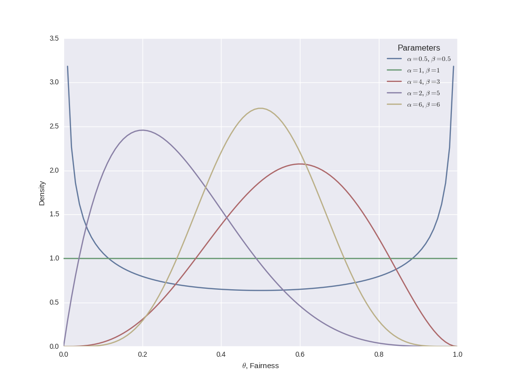
I've plotted a few separate realisations of the beta distribution for various parameters $\alpha$ and $\beta$ below:
To plot the image yourself, you will need to install seaborn:
pip install seaborn
The Python code to produce the plot is given below:
import numpy as np
from scipy.stats import beta
import matplotlib.pyplot as plt
import seaborn as sns


if __name__ == "__main__":
    sns.set_palette("deep", desat=.6)
    sns.set_context(rc={"figure.figsize": (8, 4)})
    x = np.linspace(0, 1, 100)
    params = [
        (0.5, 0.5),
        (1, 1),
        (4, 3),
        (2, 5),
        (6, 6)
    ]
    for p in params:
        y = beta.pdf(x, p[0], p[1])
        plt.plot(x, y, label="$\\alpha=%s$, $\\beta=%s$" % p)
    plt.xlabel("$\\theta$, Fairness")
    plt.ylabel("Density")
    plt.legend(title="Parameters")
    plt.show()
Essentially, as $\alpha$ becomes larger the bulk of the probability distribution moves towards the right (a coin biased to come up heads more often), whereas an increase in $\beta$ moves the distribution towards the left (a coin biased to come up tails more often).
However, if both $\alpha$ and $\beta$ increase then the distribution begins to narrow. If $\alpha$ and $\beta$ increase equally, then the distribution will peak over $\theta=0.5$, i.e. when the coin is far.
Why have we chosen the beta function as our prior? There are a couple of reasons:
- Support - It's defined on the interval $[0,1]$, which is the same interval that $\theta$ exists over.
- Flexibility - It possesses two shape parameters known as $\alpha$ and $\beta$, which give it significant flexibility. This flexibility provides us with a lot of choice in how we model our beliefs.
However, perhaps the most important reason for choosing a beta distribution is because it is a conjugate prior for the Bernoulli distribution.
Conjugate Priors
In Bayes' rule above we can see that the posterior distribution is proportional to the product of the prior distribution and the likelihood function:
\begin{eqnarray} P(\theta | D) \propto P(D|\theta) P(\theta) \end{eqnarray}A conjugate prior is a choice of prior distribution, that when coupled with a specific type of likelihood function, provides a posterior distribution that is of the same family as the prior distribution.
The prior and posterior both have the same probability distribution family, but with differing parameters.
Conjugate priors are extremely convenient from a calculation point of view as they provide closed-form expressions for the posterior, thus negating any complex numerical integration.
In our case, if we use a Bernoulli likelihood function AND a beta distribution as the choice of our prior, we immediately know that the posterior will also be a beta distribution.
Using a beta distribution for the prior in this manner means that we can carry out more experimental coin flips and straightforwardly refine our beliefs. The posterior will become the new prior and we can use Bayes' rule successively as new coin flips are generated.
If our prior belief is specified by a beta distribution and we have a Bernoulli likelihood function, then our posterior will also be a beta distribution.
Note however that a prior is only conjugate with respect to a particular likelihood function.
Why Is A Beta Prior Conjugate to the Bernoulli Likelihood?
We can actually use a simple calculation to prove why the choice of the beta distribution for the prior, with a Bernoulli likelihood, gives a beta distribution for the posterior.
As mentioned above, the probability density function of a beta distribution, for our particular parameter $\theta$, is given by:
\begin{eqnarray} P(\theta | \alpha, \beta) = \theta^{\alpha - 1} (1 - \theta)^{\beta - 1} / B(\alpha, \beta) \end{eqnarray}You can see that the form of the beta distribution is similar to the form of a Bernoulli likelihood. In fact, if you multiply the two together (as in Bayes' rule), you get:
\begin{eqnarray} \theta^{\alpha - 1} (1 - \theta)^{\beta - 1} / B(\alpha, \beta) \times \theta^{k} (1 - \theta)^{1-k} \propto \theta^{\alpha + k - 1} (1 - \theta)^{\beta + k} \end{eqnarray}Notice that the term on the right hand side of the proportionality sign has the same form as our prior (up to a normalising constant).
Multiple Ways to Specify a Beta Prior
At this stage we've discussed the fact that we want to use a beta distribution in order to specify our prior beliefs about the fairness of the coin. However, we only have two parameters to play with, namely $\alpha$ and $\beta$.
How do these two parameters correspond to our more intuitive sense of "likely fairness" and "uncertainty in fairness"?
Well, these two concepts neatly correspond to the mean and the variance of the beta distribution. Hence, if we can find a relationship between these two values and the $\alpha$ and $\beta$ parameters, we can more easily specify our beliefs.
It turns out (see this Cross Validated post and the Wikipedia article on the beta distribution) that the mean $\mu$ is given by:
\begin{eqnarray} \mu = \frac{\alpha}{\alpha + \beta} \end{eqnarray}While the standard deviation $\sigma$ is given by:
\begin{eqnarray} \sigma = \sqrt{\frac{\alpha \beta}{(\alpha + \beta)^2 (\alpha + \beta + 1)}} \end{eqnarray}Hence, all we need to do is re-arrange these formulae to provide $\alpha$ and $\beta$ in terms of $\mu$ and $\sigma$. $\alpha$ is given by:
\begin{eqnarray} \alpha = \left( \frac{1-\mu}{\sigma^2} - \frac{1}{\mu} \right) \mu^2 \end{eqnarray}While $\beta$ is given by:
\begin{eqnarray} \beta = \alpha \left( \frac{1}{\mu} - 1 \right) \end{eqnarray}Note that we have to be careful here, as we should not specify a $\sigma > 0.289$, since this is the standard deviation of a uniform density (which itself implies no prior belief on any particular fairness of the coin).
Let's carry out an example now. Suppose I think the fairness of the coin is around 0.5, but I'm not particularly certain. I may specify a standard deviation of around 0.1. What beta distribution is produced as a result?
Plugging in the numbers into the above formulae gives us $\alpha = 12$ and $\beta = 12$ and the beta distribution in this instance looks like the following:
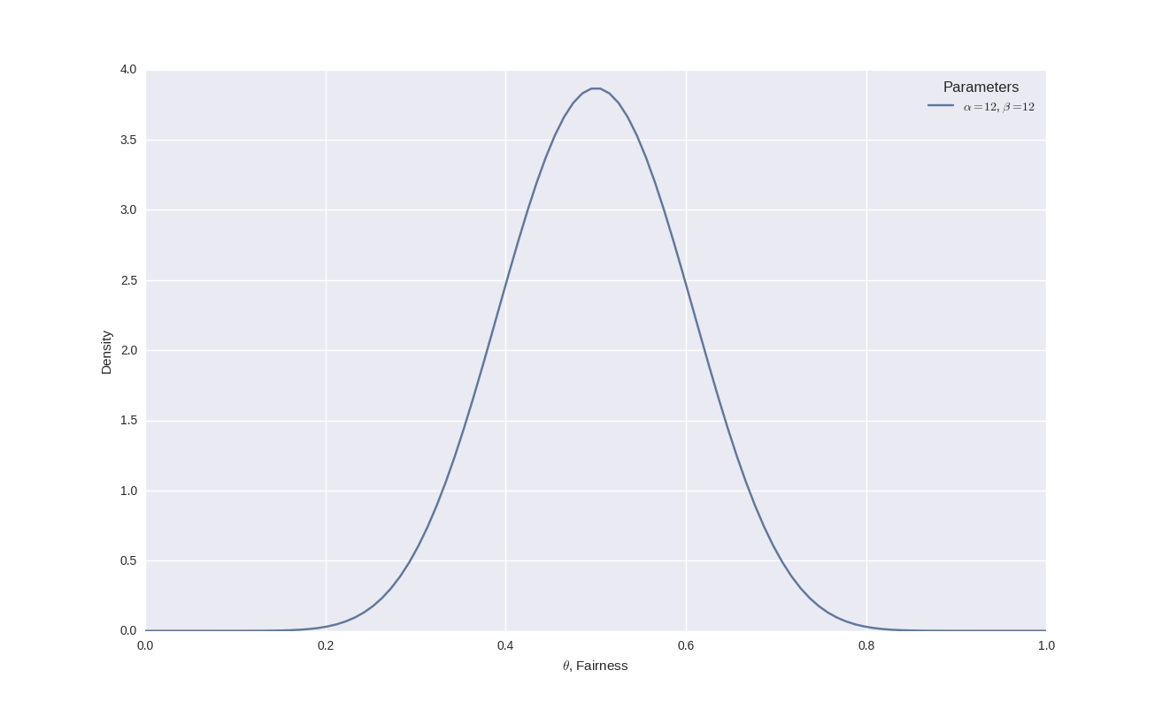
Notice how the peak is centred around 0.5 but that there is significant uncertainty in this belief, represented by the width of the curve.
Using Bayes' Rule to Calculate a Posterior
We are now finally in a position to be able to calculate our posterior beliefs using Bayes' rule.
Bayes' rule in this instance is given by:
\begin{eqnarray} P(\theta | z, N) = P(z, N | \theta) P(\theta) / P(z, N) \end{eqnarray}This says that the posterior belief in $\theta$, given $z$ heads in $N$ flips, is equal to the likelihood of seeing $z$ heads in $N$ flips, given a fairness $\theta$, multiplied by our prior belief in $\theta$, normalised by the evidence.
If we substitute in the values for the likelihood function calculated above, as well as our prior belief beta distribution, we get:
\begin{eqnarray} P(\theta | z, N) &\propto& P(z, N | \theta) P(\theta) \\ &\propto& \theta^z (1- \theta)^{N-z} \theta^{\alpha - 1} (1-\theta)^{\beta - 1} \\ &=& \theta^{z + \alpha -1} (1- \theta)^{N-z + \beta - 1} \\ &=& \text{beta}(\theta | z + \alpha, N - z + \beta) \end{eqnarray}If our prior is given by $\text{beta}(\theta|\alpha,\beta)$ and we observe $z$ heads in $N$ flips subsequently, then the posterior is given by $\text{beta}(\theta|z+\alpha, N-z+\beta)$.
This is an incredibly straightforward (and useful!) updating rule. All we need do is specify the mean $\mu$ and standard deviation $\sigma$ of our prior beliefs, carry out $N$ flips and observe the number of heads $z$ and we automatically have a rule for how our beliefs should be updated.
As an example, suppose we consider the same prior beliefs as above for $\theta$ with $\mu=0.5$ and $\sigma=0.1$. This gave us the prior belief distribution of $\text{beta}(\theta|12,12)$.
Now suppose we observe $N=50$ flips and $z=10$ of them come up heads. How does this change our belief on the fairness of the coin?
We can plug these numbers into our posterior beta distribution to get:
\begin{eqnarray} \text{beta}(\theta |z+\alpha, N-z+\beta) &=& \text{beta}(\theta |10+12, 50-10+12) \\ &=& \text{beta}(\theta |22, 52) \end{eqnarray}We can plot the prior and posterior belief distributions. I have used a blue dotted line for the prior belief and a green solid line for the posterior:
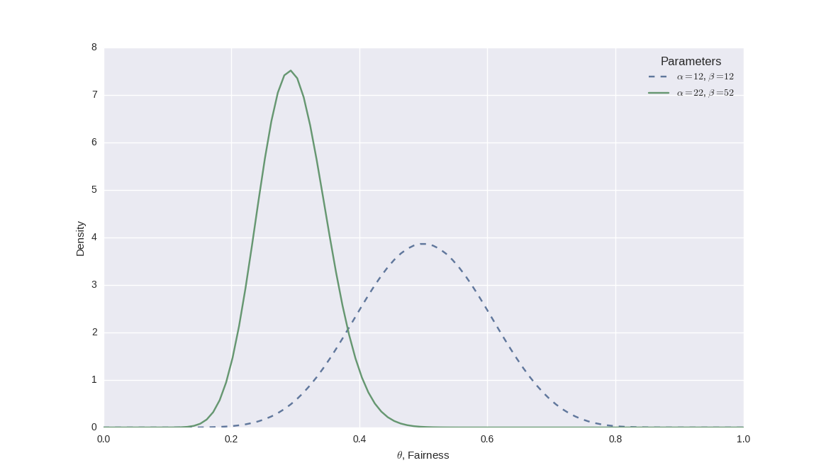
Notice how the peak shifts dramatically to the left since we have only observed 10 heads in 50 flips. In addition, notice how the width of the peak has shrunk, which is indicative of the fact that our belief in the certainty of the particular fairness value has also increased.
At this stage we can compute the mean and standard deviation of the posterior in order to produce estimates for the fairness of the coin. In particular, the value of $\mu_{\text{post}}$ is given by: \begin{eqnarray} \mu_{\text{post}} &=& \frac{\alpha}{\alpha + \beta} \\ &=& \frac{22}{22+52} \\ &=& 0.297 \end{eqnarray}
While the standard deviation $\sigma_{\text{post}}$ is given by:
\begin{eqnarray} \sigma_{\text{post}} &=& \sqrt{\frac{\alpha \beta}{(\alpha + \beta)^2 (\alpha + \beta + 1)}} \\ &=& \sqrt{\frac{22 \times 52}{(22 + 52)^2 (22 + 52 + 1)}} \\ &=& 0.053 \end{eqnarray}In particular the mean has sifted to approximately 0.3, while the standard deviation (s.d.) has halved to approximately 0.05. A mean of $\theta=0.3$ states that approximately 30% of the time, the coin will come up heads, while 70% of the time it will come up tails. The s.d. of 0.05 means that while we are more certain in this estimate than before, we are still somewhat uncertain about this 30% value.
If we were to carry out more coin flips, the s.d. would reduce even further as $\alpha$ and $\beta$ continued to increase, representing our continued increase in certainty as more trials are carried out.
Note in particular that we can use a posterior beta distribution as a prior distribution in a new Bayesian updating procedure. This is another extremely useful benefit of using conjugate priors to model our beliefs.
In the next article we are going to discuss what happens in the case where a beta distribution is insufficient to model our prior beliefs about uncertainty, in which case we will need to use a numerical method, known as Markov Chain Monte Carlo sampling, in order to construct our posterior distribution.


