Updated for Python 3.10, June 2022
In previous discussions of Bayesian Inference we introduced Bayesian Statistics and considered how to infer a binomial proportion using the concept of conjugate priors. We discussed the fact that not all models can make use of conjugate priors and thus calculation of the posterior distribution would need to be approximated numerically.
In this article we introduce the main family of algorithms, known collectively as Markov Chain Monte Carlo (MCMC), that allow us to approximate the posterior distribution as calculated by Bayes' Theorem. In particular, we consider the Metropolis Algorithm, which is easily stated and relatively straightforward to understand. It serves as a useful starting point when learning about MCMC before delving into more sophisticated algorithms such as Metropolis-Hastings, Gibbs Samplers and Hamiltonian Monte Carlo.
Once we have described how MCMC works we will carry it out using the open-source PyMC library, which takes care of many of the underlying implementation details allowing us to concentrate on Bayesian modelling.
If you have not yet looked at the previous articles on Bayesian Statistics I suggest reading the following before proceeding:
- Bayesian Statistics: A Beginner's Guide
- Bayesian Inference of a Binomial Proportion - The Analytical Approach
Bayesian Inference Goals
Our goal in carrying out Bayesian Statistics is to produce quantitative trading strategies based on Bayesian models. However, in order to reach that goal we need to consider a reasonable amount of Bayesian Statistics theory. So far we have:
- Introduced the philosophy of Bayesian Statistics, making use of Bayes' Theorem to update our prior beliefs on probabilities of outcomes based on new data
- Used conjugate priors as a means of simplifying computation of the posterior distribution in the case of inference on a binomial proportion
In this article we are going to discuss MCMC as a means of computing the posterior distribution when conjugate priors are not applicable.
Subsequent to a discussion on MCMC in this article, using PyMC, we will consider more sophisticated samplers and then apply them to more complex models. Ultimately, we will arrive at the point where our models are useful enough to provide insight into asset returns prediction. At that stage we will be able to begin building a trading model from our Bayesian analysis.
Why Markov Chain Monte Carlo?
In the previous article we considered conjugate priors, which gave us a significant mathematical "shortcut" to calculating the posterior distribution in Bayes' Rule. A perfectly legitimate question at this point would be to ask why we need MCMC at all if we can simply use conjugate priors.
The answer lies in the fact that not all models can be succinctly stated in terms of conjugate priors. In particular, many more complicated modelling situations, particularly those related to hierarchical models with hundreds of parameters, are completely intractable using analytical methods.
If we recall Bayes' Rule:
\begin{eqnarray} P(\theta | D) = \frac{P(D | \theta) P(\theta)}{P(D)} \end{eqnarray}We can see that we need to calculate the evidence $P(D)$. In order to achieve this we need to evaluate the following integral, which integrates over all possible values of $\theta$, the parameters:
\begin{eqnarray} P(D) = \int_{\Theta} P(D, \theta) \text{d}\theta \end{eqnarray}The fundamental problem is that we are often unable to evaluate this integral analytically and so we must turn to a numerical approximation method instead.
An additional problem is that our models might require a large number of parameters. This means that our prior distributions could potentially have a large number of dimensions. This in turn means that our posterior distributions will also be high dimensional. Hence, we are in a situation where we have to numerically evaluate an integral in a potentially very large dimensional space.
Thus we are in a situation often described as the Curse of Dimensionality. Informally, this means that the volume of a high-dimensional space is so vast that any available data becomes extremely sparse within that space and hence leads to problems of statistical significance. Practically, in order to gain any statistical significance, the volume of data needed must grow exponentially with the number of dimensions.
Such problems are often extremely difficult to tackle unless they are approached in an intelligent manner. The motivation behind Markov Chain Monte Carlo methods is that they perform an intelligent search within a high dimensional space and thus Bayesian Models in high dimensions become tractable.
The basic idea is to sample from the posterior distribution by combining a "random search" (the Monte Carlo aspect) with a mechanism for intelligently "jumping" around, but in a manner that ultimately doesn't depend on where we started from (the Markov Chain aspect). Hence Markov Chain Monte Carlo methods are memoryless searches performed with intelligent jumps.
As an aside, MCMC is not just for carrying out Bayesian Statistics. It is also widely used in computational physics and computational biology as it can be applied generally to the approximation of any high dimensional integral.
Markov Chain Monte Carlo Algorithms
Markov Chain Monte Carlo is a family of algorithms, rather than one particular method. In this article we are going to concentrate on a particular method known as the Metropolis Algorithm. In future articles we will consider Metropolis-Hastings, the Gibbs Sampler, Hamiltonian MCMC and the No-U-Turn Sampler (NUTS). The latter is actually incorporated into PyMC, the software we'll be using to numerically infer our binomial proportion in this article.
The Metropolis Algorithm
The first MCMC algorithm considered in this article series is due to Metropolis (1953). As you can see, it is quite an old method! While there have been substantial improvements on MCMC sampling algorithms since, it will suffice for this article. The intuition gained on this simpler method will help us understand more complex samplers in later articles.
The basic recipes for most MCMC algorithms tend to follow this pattern (see Bayesian Methods for Hackers for more details):
- Begin the algorithm at the current position in parameter space ($\theta_{\text{current}}$)
- Propose a "jump" to a new position in parameter space ($\theta_{\text{new}}$)
- Accept or reject the jump probabilistically using the prior information and available data
- If the jump is accepted, move to the new position and return to step 1
- If the jump is rejected, stay where you are and return to step 1
- After a set number of jumps have occurred, return all of the accepted positions
The main difference between MCMC algorithms occurs in how you jump as well as how you decide whether to jump.
The Metropolis algorithm uses a normal distribution to propose a jump. This normal distribution has a mean value $\mu$ which is equal to the current position and takes a "proposal width" for its standard deviation $\sigma$.
This proposal width is a parameter of the Metropolis algorithm and has a significant impact on convergence. A larger proposal width will jump further and cover more space in the posterior distribution, but might miss a region of higher probability initially. However, a smaller proposal width won't cover as much of the space as quickly and thus could take longer to converge.
A normal distribution is a good choice for such a proposal distribution (for continuous parameters) as, by definition, it is more likely to select points nearer to the current position than further away. However, it will occassionally choose points further away, allowing the space to be explored.
Once the jump has been proposed, we need to decide (in a probabilistic manner) whether it is a good move to jump to the new position. How do we do this? We calculate the ratio of the proposal distribution of the new position and the proposal distribution at the current position to determine the probability of moving, $p$:
\begin{eqnarray} p = P(\theta_{\text{new}})/P(\theta_{\text{current}}) \end{eqnarray}We then generate a uniform random number on the interval $[0,1]$. If this number is contained within the interval $[0,p]$ then we accept the move, otherwise we reject it.
While this is a relatively simple algorithm it isn't immediately clear why this makes sense and how it helps us avoid the intractable problem of calculating a high dimensional integral of the evidence, $P(D)$.
As Thomas Wiecki points out in his article on MCMC sampling, we're actually dividing the posterior of the proposed parameter by the posterior of the current parameter. Utilising Bayes' Rule this eliminates the evidence, $P(D)$ from the ratio:
\begin{eqnarray} \frac{P(\theta_{\text{new}}|D)}{P(\theta_{\text{current}}|D)} = \frac{\frac{P(D|\theta_{\text{new}})P(\theta_{\text{new}})}{P(D)}}{\frac{P(D|\theta_{\text{current}})P(\theta_{\text{current}})}{P(D)}} = \frac{P(D|\theta_{\text{new}})P(\theta_{\text{new}})}{P(D|\theta_{\text{current}})P(\theta_{\text{current}})} \end{eqnarray}The right hand side of the latter equality contains only the likelihoods and the priors, both of which we can calculate easily. Hence by dividing the posterior at one position by the posterior at another, we're sampling regions of higher posterior probability more often than not, in a manner which fully reflects the probability of the data.
Introducing PyMC
PyMC is a Python library that carries out "Probabilistic Programming". That is, we can define a probabilistic model and then carry out Bayesian inference on the model, using various flavours of Markov Chain Monte Carlo. In this sense it is similar to the JAGS and Stan packages. PyMC has a long list of contributors and is currently under active development.
PyMC has been designed with a clean syntax that allows extremely straightforward model specification, with minimal "boilerplate" code. There are classes for all major probability distributions and it is easy to add more specialist distributions. It has a diverse and powerful suite of MCMC sampling algorithms, including the Metropolis algorithm that we discussed above, as well as the No-U-Turn Sampler (NUTS). This allows us to define complex models with many thousands of parameters.
It also makes use of the Python Theano library, often used for highly CPU/GPU-intensive Deep Learning applications, in order to maximise efficiency in execution speed.
We will be taking a good look at Theano in future articles, when we come to discuss Deep Learning as applied to quantitative trading.
In this article we will use PyMC to carry out a simple example of inferring a binomial proportion, which is sufficient to express the main ideas, without getting bogged down in MCMC implementation specifics. In later articles we will explore more features of PyMC once we come to carry out inference on more sophisticated models.
Inferring a Binomial Proportion with Markov Chain Monte Carlo
If you recall from the article on inferring a binomial proportion using conjugate priors our goal was to estimate the fairness of a coin, by carrying out a sequence of coin flips.
The fairness of the coin is given by a parameter $\theta \in [0,1]$ where $\theta=0.5$ means a coin equally likely to come up heads or tails.
We discussed the fact that we could use a relatively flexible probability distribution, the beta distribution, to model our prior belief on the fairness of the coin. We also learnt that by using a Bernoulli likelihood function to simulate virtual coin flips with a particular fairness, that our posterior belief would also have the form of a beta distribution. This is an example of a conjugate prior.
To be clear, this means we do not need to use MCMC to estimate the posterior in this particular case as there is already an analytic closed-form solution. However, the majority of Bayesian inference models do not admit a closed-form solution for the posterior, and hence it is necessary to use MCMC in these cases.
We are going to apply MCMC to a case where we already "know the answer", so that we can compare the results from a closed-form solution and one calculated by numerical approximation.
Inferring a Binomial Proportion with Conjugate Priors Recap
In the previous article we took a particular prior belief that the coin was likely to be fair, but that we weren't particularly certain. This translated as giving $\theta$ a mean $\mu=0.5$ and a standard deviation $\sigma=0.1$.
A beta distribution has two parameters, $\alpha$ and $\beta$, that characterise the "shape" of our beliefs. A mean $\mu=0.5$ and s.d. $\sigma=0.1$ translate into $\alpha=12$ and $\beta=12$ (see the previous article for details on this transformation).
We then carried out 50 flips and observed 10 heads. When we plugged this into our closed-form solution for the posterior beta distribution, we received a posterior with $\alpha=22$ and $\beta=52$. I've replotted the figure showing the two distributions here:
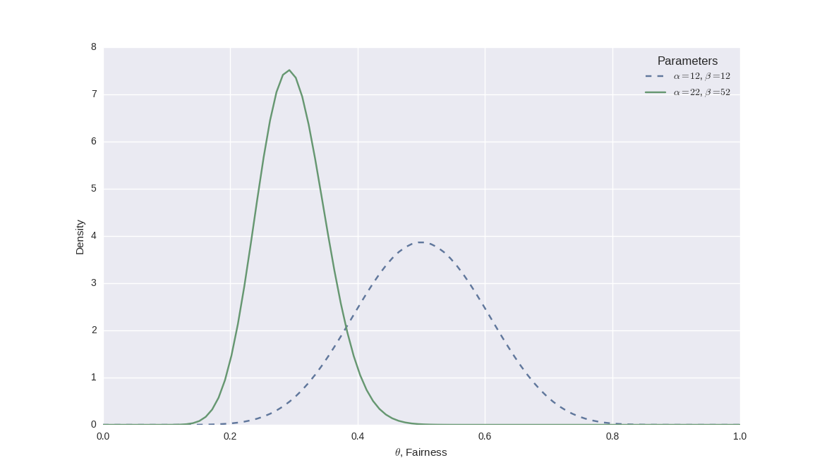
We can see that this intuitively makes sense, as the mass of probability has dramatically shifted to nearer 0.2, which is the sample fairness from our flips. Notice also that the peak has become narrower as we're quite confident in our results now, having carried out 50 flips.
Inferring a Binonial Proportion with PyMC
We're now going to carry out the same analysis using the numerical Markov Chain Monte Carlo method instead.
Firstly, we need to install PyMC. Please install as recommended by the documentation. For Linux, Windows and MacOSX it is recommended to use Anaconda and install into a virtul environment. Below is the code to carry out this installation using the Anaconda package manager conda. In this code snippet we create a virtual environment named pymc_env and install the current versions of Python and PyMC directly into it.
conda create -c conda-forge -n pymc_env python pymc
This will install all the necessary packages required for PyMC to work. These include but are not limited to (at time of writing) Python 3.10, Matplotlib-base 3.5, Numpy 1.22 and Scipy 1.7. Once installed you will need to activate the environment you have just created.
conda activate pymc_env
The next task is to import the necessary libraries, which include Matplotlib, Numpy, Scipy and PyMC itself. We also set the graphical style of the Matplotlib output to be similar to the ggplot2 graphing library from the R statistical language:
import matplotlib.pyplot as plt
import numpy as np
import pymc
import scipy.stats as stats

plt.style.use("ggplot")
The next step is to define our main function and set our prior parameters, as well as the number of coin flip trials carried out and heads returned. We also specify, for completeness, the parameters of the analytically-calculated posterior beta distribution, which we will use for comparison with our MCMC approach. In addition we specify that we want to carry out 100,000 iterations of the Metropolis algorithm:
if __name__ == '__main__':

    # Parameter values for prior and analytic posterior
    n = 50
    z = 10
    alpha = 12
    beta = 12
    alpha_post = 22
    beta_post = 52

    # How many iterations of the Metropolis
    # algorithm to carry out for MCMC
    iterations = 100000
Now we actually define our beta distribution prior and Bernoulli likelihood model. PyMC has a very clean API for carrying this out. It uses a Python with context to assign all of the parameters, step sizes and starting values to a pymc.Model instance (which I have called basic_model, as per the PyMC tutorial).
Firstly, we specify the theta parameter as a beta distribution, taking the prior alpha and beta values as parameters. Remember that our particular values of $\alpha=12$ and $\beta=12$ imply a prior mean $\mu=0.5$ and a prior s.d. $\sigma=0.1$.
We then define the Bernoulli likelihood function, specifying the fairness parameter p=theta, the number of trials n=n and the observed heads observed=z, all taken from the parameters specified above.
At this stage we can find an optimal starting value for the Metropolis algorithm using the PyMC Maximum A Posteriori (MAP) optimisation (we will go into detail about this in later articles). Finally we specify the Metropolis sampler to be used and then actually sample(..) the results. These results are stored in the trace variable:
def create_mcmc_model(alpha, beta, n, z, iterations):
    # Use PyMC to construct a model context
    with pm.Model() as basic_model:
        # Define our prior belief about the fairness
        # of the coin using a Beta distribution
        theta = pm.Beta("theta", alpha=alpha, beta=beta)

        # Define the Bernoulli likelihood function
        y = pm.Binomial("y", n=n, p=theta, observed=z)

        # Carry out the MCMC analysis using the Metropolis algorithm
        # Use Maximum A Posteriori (MAP) optimisation as initial value for MCMC
        start = pm.find_MAP()

        # Use the Metropolis algorithm (as opposed to NUTS or HMC, etc.)
        step = pm.Metropolis()

        # Calculate the trace
        trace = pm.sample(
            draws=iterations,
            step=step,
            init=start,
            chains=1,
            random_seed=1,
            progressbar=True
        )
    return trace
Notice how the specification of the model via the PyMC API is almost akin to the actual mathematical specification of the model, with minimal "boilerplate" code. We will demonstrate the power of this API in later articles when we come to specify some more complex models.
Now that the model has been specified and sampled, we wish to plot the results. The trace object is a MultiTrace or ArviZ InferenceData object that contains the samples. The inference data is divided into the following groups.
- posterior
- log_likelihood
- sample_stats
- observed_data
Each one of these groups contains further information about the model we have created. The list of all the accepted samples from the MCMC sampling can be found by calling posterior.theta This returns an xarray.DataArray with a list for the data from each chain that has been run. In order to plot the data with Matplotlib we must first export the 0th list in this xarray.DataArray to a numpy array. If we use dir(trace.posterior.theta) we can see that the theta object has a to_numpy() method. So in order to access the data we need to use trace['posterior']['theta'][0].to_numpy().
We can now create a histogram from the list of all accepted samples of the MCMC sampling using 50 bins, we will add these as a variable in our main function in the next step. We then plot the analytic prior and posterior beta distributions using the SciPy stats.beta.pdf(..) method. Finally, we add some labelling to the graph and display it:
def plot_mcmc_comparison(trace, bins, alpha, beta, alpha_post, beta_post):
    # Plot the posterior histogram from MCMC analysis
    plt.hist(
        trace['posterior']['theta'][0].to_numpy(), bins,
        histtype="step", density=True,
        label="Posterior (MCMC)", color="red"
    )

    # Plot the analytic prior and posterior beta distributions
    x = np.linspace(0, 1, 100)
    plt.plot(
        x, stats.beta.pdf(x, alpha, beta),
        "--", label="Prior", color="blue"
    )
    plt.plot(
        x, stats.beta.pdf(x, alpha_post, beta_post),
        label='Posterior (Analytic)', color="green"
    )

    # Update the graph labels
    plt.legend(title="Parameters", loc="best")
    plt.xlabel("$\\theta$, Fairness")
    plt.ylabel("Density")
    plt.show()

    # Display the plot
    plt.show()
The last thing we need to do is to update our __main__ function to include the histogram bins and to call our functions.
if __name__ == '__main__':

    # Parameter values for prior and analytic posterior
    n = 50
    z = 10
    alpha = 12
    beta = 12
    alpha_post = 22
    beta_post = 52

    # How many iterations of the Metropolis
    # algorithm to carry out for MCMC
    iterations = 100000

    # Number of Bins for Histogram
    bins=50

    mcmc_model = create_mcmc_model(alpha, beta, n, z, iterations)
    plot_mcmc_comparison(mcmc_model, bins, alpha, beta, alpha_post, beta_post)
When the code is executed the following output is given:
 [----------------------------] 100.00% [6/6 00:00<00:00 logp = -10.252, ||grad|| = 15]]
Sequential sampling (1 chains in 1 job)
Metropolis: [theta]
Sampling 1 chain for 1_000 tune and 100_000 draw iterations (1_000 + 100_000 draws total) took 30 seconds.]
Clearly, the sampling time will depend upon the speed of your computer. The graphical output of the analysis is given in the following image:
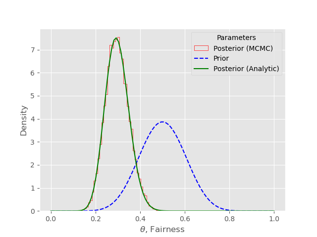
In this particular case of a single-parameter model, with 100,000 samples, the convergence of the Metropolis algorithm is extremely good. The histogram closely follows the analytically calculated posterior distribution, as we'd expect. In a relatively simple model such as this we do not need to compute 100,000 samples and far fewer would do. However, it does emphasise the convergence of the Metropolis algorithm.
We can also consider a concept known as the trace, which is the vector of samples produced by the MCMC sampling procedure. We can use the helpful plot_trace() method to plot both a kernel density estimate (KDE) of the histogram displayed above, as well as the trace.
The trace plot is extremely useful for assessing convergence of an MCMC algorithm and whether we need to exclude a period of initial samples (known as the burn in). We will discuss the trace, burn in and other convergence issues in future articles when we study more sophisticated samplers. To output the trace we simply call plot_trace() with the trace variable:
# Show the trace plot
pm.plot_trace(trace)
plt.show()
Here is the full trace plot:

As you can see, the KDE estimate of the posterior belief in the fairness reflects both our prior belief of $\theta=0.5$ and our data with a sample fairness of $\theta=0.2$. In addition we can see that the MCMC sampling procedure has "converged to the distribution" since the sampling series looks stationary.
In more complicated cases, which we will examine in later articles, we will see that we need to consider a "burn in" period as well as "thin" the results to remove autocorrelation, both of which will improve convergence.
For completeness, here is the full listing:
import matplotlib.pyplot as plt
import numpy as np
import pymc as pm
import scipy.stats as stats

plt.style.use("ggplot")


def create_mcmc_model(alpha, beta, n, z, iterations):
    # Use PyMC to construct a model context
    with pm.Model() as basic_model:
        # Define our prior belief about the fairness
        # of the coin using a Beta distribution
        theta = pm.Beta("theta", alpha=alpha, beta=beta)

        # Define the Bernoulli likelihood function
        y = pm.Binomial("y", n=n, p=theta, observed=z)

        # Carry out the MCMC analysis using the Metropolis algorithm
        # Use Maximum A Posteriori (MAP) optimisation as initial value for MCMC
        start = pm.find_MAP()

        # Use the Metropolis algorithm (as opposed to NUTS or HMC, etc.)
        step = pm.Metropolis()

        # Calculate the trace
        trace = pm.sample(
            draws=iterations,
            step=step,
            init=start,
            chains=1,
            random_seed=1,
            progressbar=True
        )
    return trace


def plot_mcmc_comparison(trace, bins, alpha, beta, alpha_post, beta_post):
    # Plot the posterior histogram from MCMC analysis
    plt.hist(
        trace['posterior']['theta'][0].to_numpy(), bins,
        histtype="step", density=True,
        label="Posterior (MCMC)", color="red"
    )

    # Plot the analytic prior and posterior beta distributions
    x = np.linspace(0, 1, 100)
    plt.plot(
        x, stats.beta.pdf(x, alpha, beta),
        "--", label="Prior", color="blue"
    )
    plt.plot(
        x, stats.beta.pdf(x, alpha_post, beta_post),
        label='Posterior (Analytic)', color="green"
    )

    # Update the graph labels
    plt.legend(title="Parameters", loc="best")
    plt.xlabel("$\\theta$, Fairness")
    plt.ylabel("Density")
    plt.show()

    # Show the trace plot
    pm.traceplot(trace)
    plt.show()


if __name__ == '__main__':

    # Parameter values for prior and analytic posterior
    n = 50
    z = 10
    alpha = 12
    beta = 12
    alpha_post = 22
    beta_post = 52

    # How many iterations of the Metropolis
    # algorithm to carry out for MCMC
    iterations = 100000

    # Number of Bins for Histogram
    bins=50

    mcmc_model = create_mcmc_model(alpha, beta, n, z, iterations)
    plot_mcmc_comparison(mcmc_model, bins, alpha, beta, alpha_post, beta_post)
Next Steps
At this stage we have a good understanding of the basics behind MCMC, as well as a specific method known as the Metropolis algorithm, as applied to inferring a binomial proportion.
However, as we discussed above, PyMC uses a much more sophisticated MCMC sampler known as the No-U-Turn Sampler (NUTS). In order to gain an understanding of this sampler we eventually need to consider further sampling techniques such as Metropolis-Hastings, Gibbs Sampling and Hamiltonian Monte Carlo (on which NUTS is based).
We also want to start applying Probabilistic Programming techniques to more complex models, such as hierarchical models. This in turn will help us produce sophisticated quantitative trading strategies.
Bibliographic Note
The algorithm described in this article is by Metropolis (1953). An improvement by Hastings (1970) led to the Metropolis-Hastings algorithm which we will discuss in a future article. The Gibbs sampler is due to Geman and Geman (1984). Gelfand and Smith (1990) wrote a paper that was considered a major starting point for extensive use of MCMC methods in the statistical community.
The Hamiltonian Monte Carlo approach is due to Duane et al (1987) and the No-U-Turn Sampler (NUTS) is due to Hoffman and Gelman (2011). Gelman et al (2013) has an extensive discussion of computional sampling mechanisms for Bayesian Statistics, including a detailed discussion on MCMC. A gentle, mathematically intuitive, introduction to the Metropolis Algorithm is given by Kruschke (2014).
A very popular on-line introduction to Bayesian Statistics is Probabilistic Programming and Bayesian Methods for Hackers by Cam Davidson-Pilon and others, which has a fantastic chapter on MCMC (and PyMC). Thomas Wiecki has also written a great blog post explaining the rationale for MCMC.
The PyMC project also has some extremely useful documentation and some examples.
References
- Davidson-Pilon, C. et al (2016) "Probabilistic Programming & Bayesian Methods for Hackers", http://camdavidsonpilon.github.io/Probabilistic-Programming-and-Bayesian-Methods-for-Hackers/
- Duane, S. et al (1987) "Hybrid Monte Carlo", Physics Letters B 195 (2): 216–222
- Gelfand, A.E. and Smith, A.F.M. (1990) "Sampling-based approaches to calculating marginal densities", J. Amer. Statist. Assoc., 85, 140, 398-409.
- Geman, S. and Geman, D. (1984) "Stochastic relaxation, Gibbs distributions and the Bayesian restoration of images.", IEEE Trans. Pattern Anal. Mach. Intell., 6, 721-741.
- Gelman, A. et al (2013) Bayesian Data Analysis, 3rd Edition, Chapman and Hall/CRC
- Hastings, W. (1970) "Monte Carlo sampling methods using Markov chains and their application", Biometrika, 57, 97-109.
- Hoffman, M.D., and Gelman, A. (2011) "The No-U-Turn Sampler: Adaptively Setting Path Lengths in Hamiltonian Monte Carlo, arXiv:1111.4246 [stat.CO]
- Kruschke, J. (2014) Doing Bayesian Data Analysis, Second Edition: A Tutorial with R, JAGS, and Stan, Academic Press
- Metropolis, N. et al (1953) "Equations of state calculations by fast computing machines", J. Chem. Phys., 21, 1087-1092.
- Robert, C. and Casella, G. (2011) "A Short History of Markov Chain Monte Carlo: Subjective Recollections from Incomplete Data", Statistical Science 0, 00, 1-14.
- Wiecki, T. (2015) "MCMC sampling for dummies", https://twiecki.github.io/blog/2015/11/10/mcmc-sampling/