Quantitative finance is an extremely competitive field at the institutional level. Quant hedge funds vie for large allocations and must continually prove their worth in order to receive new assets under management. This drives a significant internal R&D effort to achieve new sources of uncorrelated risk-adjusted returns for their clients. Funds and their trading desks must continually hunt for new sources of alpha. This can sometimes be found in new markets, with innovative data sources or with better predictive algorithms.

In recent years much of the quantitative hedge fund industry has turned its attention towards so-called alternative data as a means of generating new alpha. Such data is often in unstructured formats unsuitable for traditional time series based modelling approaches. Hence there is a strong push to leverage mechanisms that can extract value from these datasets and use them for predictive signal generation. One such field that has garnered significant attention in recent years is that of deep learning.

To discover more about deep learning please read our previous article: What Is Deep Learning?

Deep learning hasn't escaped the attention of the practitioner retail quant either. The explosive rise of powerful open source software, along with the ever growing availability of data, combined with cheap access to computational hardware has lead many retail quants to pursue trading strategies powered by deep learning models.

Despite the relative simplicity of the APIs provided by modern deep learning frameworks there is still a substantial learning curve to be overcome in order to be able to successfully carry out quantitative trading research using deep learning approaches.

As with any complex predictive model it is insufficient to simply 'copy and paste' open source model code and hope to generate a solid trading strategy. Instead a good understanding of the underlying models are required in order to avoid common pitfalls such as overfitting.

In this new series of articles we are going to explore deep learning models, first by studying the theory of the common models and subsequently by providing robust implementations that can be utilised and extended for your own trading purposes.

It is common for many deep learning tutorials to jump straight into code. While this is a useful learning approach for relatively simple examples, such as classifying objects in images, it is less appropriate in the realm of quantitative finance, where model errors can lead to significant unprofitability.

For this reason QuantStart will emphasise both theory and practice in order to provide a well-rounded understanding of the field and to help mitigate trading losses by deploying poorly constructed models.

This article will begin by introducing artificial neural network (ANN) models. It will discuss how they are inspired by biological neural networks. Attention will then turn to one of the earliest neural network models, known as the perceptron.

In future articles we will use the perceptron model as a 'building block' towards the construction of more sophisticated deep neural networks such as multi-layer perceptrons (MLP), demonstrating their power on some non-trivial machine learning problems.

Artificial Neural Networks

Deep learning may seem like an extremely modern field but research into the area began in the 1940s. In much the same way that birds have always motivated humans to develop heavier-than-air flight, the architecture of the human brain has motivated humans to try and replicate intelligence via similar neural structures.

The neuron itself provided the inspiration for the development of networks of computational neurons, which can be combined to produce sophisticated computation even from fairly simple network architectures.

The arrangement of the human cerebral cortex has also been a significant motivator in certain deep neural network architectures such as the Convolutional Neural Network (CNN), which will be the focus of future articles.

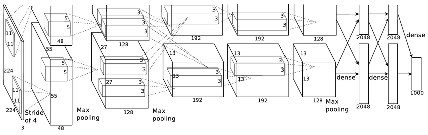
"AlexNet" Convolutional Neural Network architecture^[4]

Research on networks of computational neurons, or artificial neural networks has been characterised by periods of intense development and funding along with relatively dormant periods known as 'AI Winters' where the promises of such technology often never lived up to the current hype.

In part this can be attributed to insufficiently complex models that were difficult to train in a reasonable time frame. The expense of obtaining, storing and processing the large quantities of data required to obtain good results was another contributing factor.

In recent years the above challenges have largely been surmounted. This has driven explosive growth in ANN research. The advent of the Graphics Processing Unit (GPU) provided the mechanism for cheap training. The rise of the internet lead to staggering quantities of easily available data. Training algorithms have steadily improved, as have model architectures.

The confluence of these achievements has produced state-of-the-art results by deep learning models on many challenging problems previously considered intractable.

While the research history of artificial neural networks is a fascinating topic in its own right, our goal here is to utilise these tools as quantitative trading practitioners in order to generate superior risk-adjusted returns. Such historical developments are out of scope for this article.

For those who wish to delve more deeply into the historical developments of artificial neural networks, please see the section Historical Trends in Deep Learning within the Deep Learning^[1] book.

We will begin our discussion of ANNs via one of the simplest possible models known as the perceptron.

The Perceptron

In this section we are going to introduce the perceptron^[2]. It is one of the earliest—and most elementary—artificial neural network models. The perceptron is extremely simple by modern deep learning model standards. However the concepts utilised in its design apply more broadly to sophisticated deep network architectures.

The perceptron is a supervised learning binary classification algorithm, originally developed by Frank Rosenblatt in 1957. It categorises input data into one of two separate states based a training procedure carried out on prior input data.

The Perceptron

The perceptron attempts to partition the input data via a linear decision boundary. A similar procedure is carried out by another supervised learning algorithm known as support vector classifiers, which you can read about in our detailed article here.

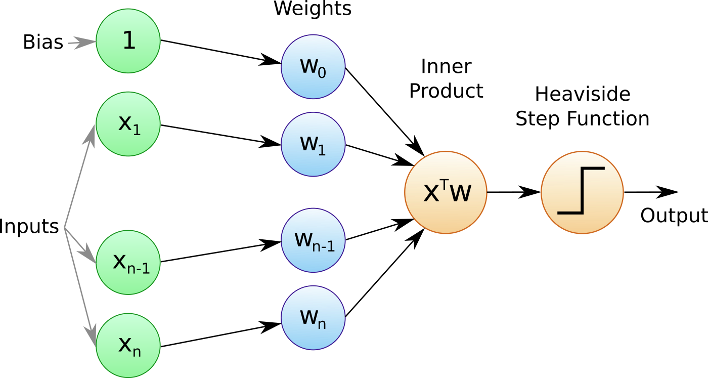
The perceptron works by taking a set of scalar input features, along with a constant 'bias' term and assigning weights to these inputs. The linear combination of the weights and inputs are taken. This linear combination is then fed through an activation function that determines which state (or class) the set of inputs belongs to.

Activation Functions for the Perceptron

In this case of the perceptron model the chosen activation function is a step function that returns one of two distinct values (three in the case of the Sign function below) depending upon the value of the linear combination.

Common choices for the step function in perceptrons are the Heaviside function and the Sign function.

The Heaviside function (named after Oliver Heaviside) is given below:

\begin{eqnarray} h(z) = \begin{cases} 0 & \text{if $z < 0$} \\ 1 & \text{if $z \geq 0$} \end{cases} \end{eqnarray}

It says that if the provided linear combination $z$ is less than 0 then simply return 0, otherwise return 1.

The Sign function is given below:

\begin{eqnarray} \text{sgn}(z) = \begin{cases} -1 & \text{if $z < 0$} \\ 0 & \text{if $z = 0$} \\ 1 & \text{if $z > 0$} \end{cases} \end{eqnarray}

It says that if the provided linear combination $z$ is less than 0 then return -1, if it is 0 then return 0, otherwise return +1.

Algorithm for the Perceptron

The mathematical procedure for determining the class label of a provided set of input data is as follows:

1. For an input vector ${\bf x}$, with components given by $x_i$, $i \in \{1,\ldots,n\}$ take the inner product of ${\bf x}$ and the weight vector ${\bf w}$ to produce the weighted sum of inputs ${\bf x}^T {\bf w}$.
2. Add the bias term, $b$ to this weighted sum to get $z = {\bf x}^T {\bf w} + b$.
3. Apply the appropriate step function to $z$ in order to determine the class label of the inputs.

The algorithm for the perceptron, when utilising the Heaviside activation function is summarised in the following function:

\begin{eqnarray} f(z) = \begin{cases} 1 & \text{if ${\bf x}^T {\bf w} + b > 0$} \\ 0 & \text{otherwise} \end{cases} \end{eqnarray}

This simply says that if the weighted sum of the inputs (including the bias) exceeds zero then classify the input as state label 1, otherwise classify it as state label 0.

Note that some references will add the bias term into the weight vector ${\bf w}$ by adding a $w_0$ component. To make this work it will be necessary to add an $x_0$ component to the input vector, which is simply always set to one: $x_0=1$. It is then possible to write the algorithm as:

\begin{eqnarray} f(z) = \begin{cases} 1 & \text{if ${\bf x}^T {\bf w} > 0$} \\ 0 & \text{otherwise} \end{cases} \end{eqnarray}

While this notation is certainly neater it should always be kept in mind that an implicit bias term exists as one of the components of this weighted sum.

Why Do We Need a Bias Term?

At this stage it may be worth asking why a bias term is needed at all? Geometrically it is possible to think of the linear decision boundary as a line (or hyperplane) that divides a region into two separate mutually exclusive subregions.

If a bias term was not present then this line (or hyperplane) would be forced to intersect the origin of the region. This could significantly reduce its predictive performance (or even render it useless) if the 'true' decision boundary did not lie on the origin. Hence it is always necessary to include a bias term to account for this possibility.

Next Steps

While the above classification algorithm provides a clear procedure on how to classify input data it does not provide any insight into how to set the weights (or bias) to allow the algorithm to proceed.

The next article in the series will discuss how perceptrons are trained so as to determine an optimal set of weights and biases for use in linear classification.

Once we have outlined the training procedure we will begin 'stacking' perceptrons together to form multi-layer perceptrons that can be used for regression and classification problems.

References

• [1] Goodfellow, I.J., Bengio, Y., Courville, A. (2016) Deep Learning, MIT Press
• [2] Rosenblatt, F. (1958). The perceptron: A probabilistic model for information storage and organization in the brain. Psychological Review, 65, 386-408.
• [3] Géron, A. (2019) Hands-On Machine Learning with Scikit-Learn, Keras, and TensorFlow, 2nd Ed., O'Reilly Media
• [4] Krizhevsky, A., Sutskever, I., Hinton, G. (2012) "ImageNet Classification with Deep Convolutional Neural Networks", Advances in Neural Information Processing Systems 25 (NIPS 2012)