In this article series QuantStart returns to the discussion of pricing derivative securities, a topic which was covered a few years ago on the site through an introduction to stochastic calculus.
Imanol Pérez, a PhD researcher in Mathematics at Oxford University, and an expert guest contributor to QuantStart describes how Lévy processes can be utilised to make the Black-Scholes model more accurate.
A standard assumption when pricing derivatives is that stock prices follow a geometric Brownian motion. In other words, these models assume that the log returns of the underlying stock are normally distributed. This assumption simplifies the model significantly, and allows us to derive the Black-Scholes formula with relative ease. Although this assumption may be good enough in some applications, the truth is that it is not a completely accurate description of market behaviour.
| Index | Mean | SD | Skewness | Kurtosis |
|---|---|---|---|---|
| S&P500 | 0.0009 | 0.0119 | -0.4409 | 6.94 |
| Nasdaq Composite | 0.0015 | 0.0154 | -0.5439 | 5.78 |
| DAX | 0.0012 | 0.0157 | -0.4314 | 4.65 |
| SMI | 0.0009 | 0.0141 | -0.3584 | 5.35 |
| CAC 40 | 0.0013 | 0.0143 | -0.2116 | 4.63 |
Table 1 - Mean, standard deviation, skewness and kurtosis of the log returns of some major indices from 1997 to 1999. Table obtained from Schoutens[4].
Take a look to Table 1 for instance. The table contains the mean, standard deviation, skewnewss and kurtosis of the log returns of S&P 500, Nasdaq Composite, DAX, SMI and CAC 40. If log returns were normally distributed, the skewness would be zero, while the kurtosis would be 3. The table shows evidence against this, as skewness and kurtosis differ significantly from the normal case. This also implies that log returns have fatter tails than if they were normally distributed.
Therefore, although the normality assumption has proved to be useful and practical sometimes, it doesn't hold in real markets.
Lévy processes
In this article, we will explore markets that are driven by Lévy processes. A stochastic process $(X_t,t\geq 0)$ is said to be a Lévy process if the following holds:
- $X_0=0$ almost surely.
- It has independent increments.
- It has stationary increments.
- It is continuous in probability, that is, given $\epsilon>0$ and $t\geq 0$, $\lim_{h\rightarrow 0} \mathbb{P}[|X_{t+h}-X_t|>\epsilon]=0$.
Notice that no normality was used to define such processes. It is also clear that the Brownian motion is a special case of a Lévy process. Other examples include the Poisson Process, the Gamma Process, etc.
Our assumption will be that the price of a stock $S$ is given by
$$S_t = S_0 \exp(X_t),$$ with $X$ some Lévy process. Over the last few decades, many choices of $X$ have been discussed. For example, Madan and Seneta[2], [3] suggested a Variance Gamma process, Barndoff-Nielsen[1] proposed a Normal-inverse Gaussian process, and some other choices were also studied.
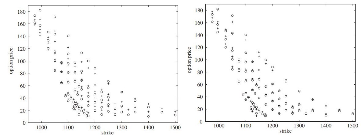
Fig 1 - Option calibration of S&P 500 options using the Black-Scholes model (left) and a Lévy-process-based model (right). Circles indicate market prices, and crosses represent model prices. Figure from Schoutens[4].
Different choices lead to different models, that can significantly improve the Black-Scholes model. For instance, consider Figure 1. It shows how accurate model prices were, when the Black-Scholes model is considered, in contrast with a Lévy process model. It is clear that model prices using a Lévy market model are better predictions that the ones provided by the Black-Scholes model, suggesting real incentives in using Lévy processes other than Brownian motions as drivers of the market. Wim Schoutens' Lévy Processes in Finance[4] is a great reference to learn more about financial derivatives pricing using Lévy processes.
Article Series
- Derivatives Pricing I: Pricing Under the Black-Scholes Model
- Derivatives Pricing II: Volatility is Rough
- Derivatives Pricing III: Models Driven By Lévy Processes
References
- [1] Barndoff-Nielsen, O.E. "Normal inverse Gaussian distributions and the modeling of stock returns", Research Report no. 300, Department of Theoretical Statistics, Aarhus University
- [2] Madan, D.B. and Seneta, E. (1987) "Chebyshev polynomial approximations and characteristic function estimation", Journal of the Royal Statistical Society B 49(2), 163-169.
- [3] Madan, D.B. and Seneta, E. (1998) "The variance Gamma process and option pricing", European Finance Review 2, 79-105.
- [4] Schoutens, W. (2003) Lévy Processes in Finance, Wiley