In this article, I will talk about how to write Monte Carlo simulations in CUDA. More specifically, I will explain how to carry it out step-by -step while writing the code for pricing a down-and-out barrier option, as its path dependency will make it a perfect example for us to learn Monte Carlo in CUDA. Also, I will show you how to efficiently generate random numbers with CUDA and how to measure performance with just a few lines of code.
First, I will start with a brief theoretical introduction so if you already know how Monte Carlo methods and barrier options work, you can skip the following sections.
Barrier Options
A barrier option is an exotic derivative, part of the set of path-dependent options, whose payoff depends not only on the underlying price at maturity but also on whether the price line hit a pre-determined level.
There are different ways to determine this level and how the price can or cannot reach it. The first is the barrier level position in relation to the current underlying price (spot), so we have a first categorization "up" or "down". The second criterion can be "in" or "out", and it refers to what happens when the event "hit the level" is triggered.
"In" means that the option starts to be active after having touched the barrier level. "Out" is the opposite, meaning that after triggering the event the option is no longer valid. Also, it could be "paired" with any kind of option. We could have a European option with barrier, as well as an American or an Asian one. Let's consider an example now.
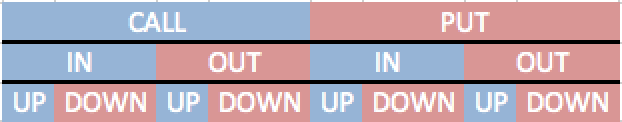
Suppose that we have a European option with a barrier. We can have any combination between call and put, in and out, up and down, which give us a total of $2^3 = 8$ different possible combinations, as we can see in the following table:
Let's choose now a down-and-out call. That means that the barrier is currently lower than the spot price and our option is already active. As we can see in the following chart:
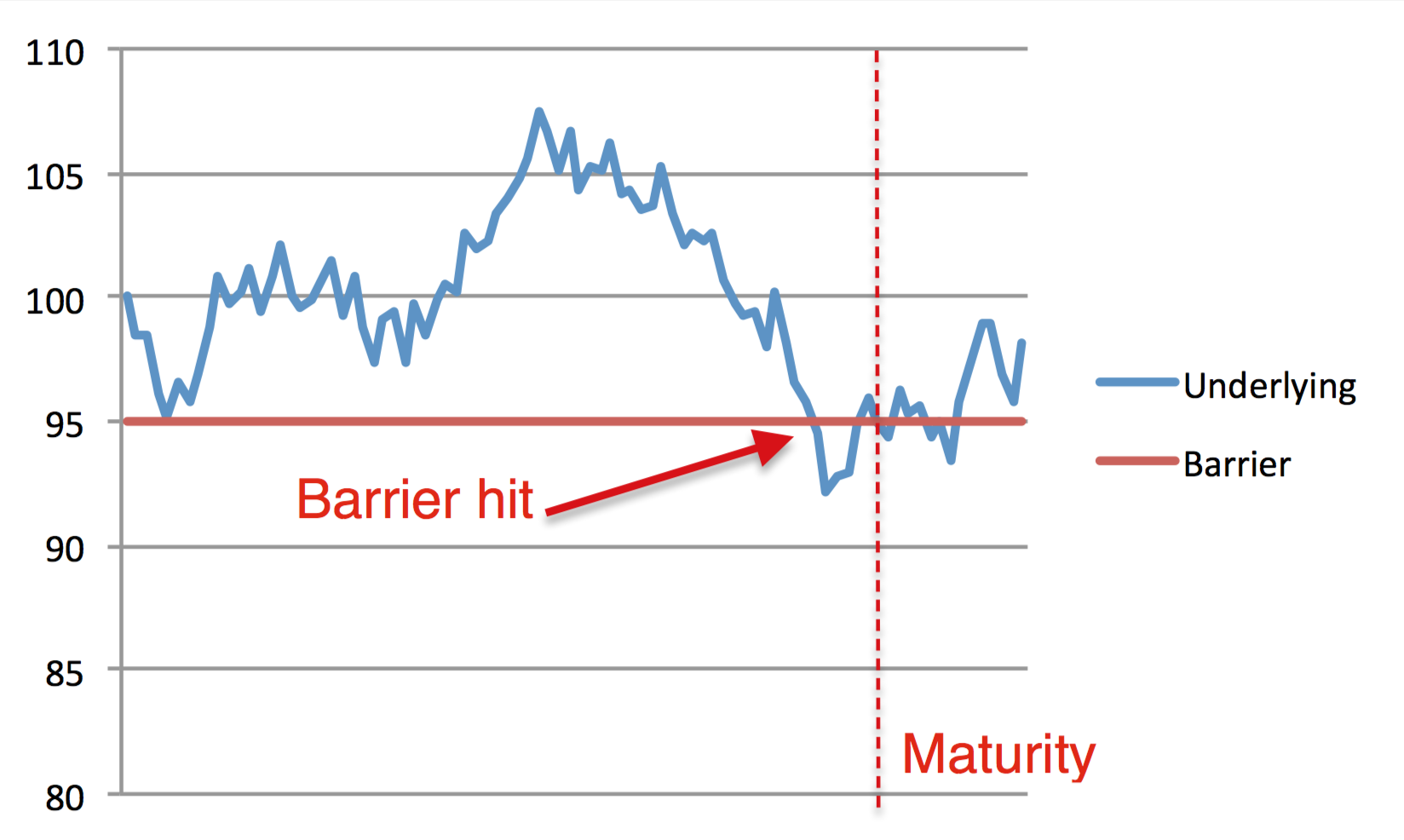
The underlying price hits the barrier before the maturity making it invalid. Sometimes, as a kind of insurance, we can have a rebate price, which is a fixed amount of money, usually less than the option value, which we will receive in case our option expires due to hitting the barrier. Of course, this will also change the price of the option itself.
In this article we will consider down-and-out barrier options without rebate, so that the payoff is given by:
\begin{eqnarray} (S_T - K)_{+},\;\; \text{if}\; S_t > B \;\; \forall t \leq T \\ R = 0, \;\; \text{if}\; S_t \leq B \;\;\ \text{for at least one}\; t < T \end{eqnarray}where $R$ is the rebate price and $B$ the barrier level.
Monte Carlo Method
The Monte Carlo method is a well-known method in finance, as it lets us compute difficult, if not impossible, expected values of complex stochastic functions. Mike has already discussed the method in several articles regarding option pricing, but a few recap lines can be helpful for those that are new to it.
The Monte Carlo method was first introduced in the field of physics, for complex simulations, very likely by Enrico Fermi in the 1930s for studying neutron diffusion. It then became popular in the 1940s among physicists and mathematicians involved in creating bombs for the U.S. Army. The projects needed a code name, so John Von Neumann chose "Monte Carlo", referring to the famous Monte Carlo Casino. Since then, technology and especially computational power have increased dramatically, letting us use these methods for a large variety of problems.
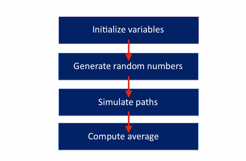
In finance the Monte Carlo method is mainly used for option pricing as, especially with exotic options, the payoff is sometimes too complex, if not impossible, to compute. The main idea behind it is quite simple: simulate the stochastic components in a formula and then average the results, leading to the expected value. Of course, the more simulations (paths) you make, the more accurate the result will be. A commonly accepted value for the minimum number of paths is $10^6$. That should give good results for most of the simulations. Otherwise, there are techniques that can reduce variance in order to make even more accurate predictions.
Given the random nature of this process, variance reduction is not the only problem we can encounter. Another one, probably the most important, is how the random numbers are generated. There is an entire branch of mathematics talking about this and a detailed explanation is well beyond the purpose of this article, but we will see that CUDA can provide different efficient methods for generating random numbers by including the useful library curand.
Monte Carlo and the GPU
As the Monte Carlo method is basically a way to compute expected values by generating random scenarios and then averaging them, it is actually very efficient to parallelise. Moreover, with consumer CPUs on standard computers it is just not possible to reach the accuracy needed, as simulating over one million paths is usually very time consuming. With the GPU we can reduce this problem by parallelising the paths. That is, we can assign each path to a single thread, simulating thousands of them in parallel, with massive savings in computational power and time. At the end of this article I will show you the numerical results, making it quite obvious why it's better to run a Monte Carlo on a GPU.
Monte Carlo and Path Dependency
First, let's see what and how to parallelise. In option pricing, usually the only variable that can assume random values is the underlying, so we only have to write a kernel that can generate a simulated value for the underlying and then calculate the option price. That's it. Sounds easy, but actually we have to cope with a couple of issues that we could have avoided for the pricing of a path-independent option.
That is, as the barrier can be hit at any point in time we have to simulate step by step the changes in the underlying price, significantly reducing the code speed. Why? Let's say that we want to run an accurate Monte Carlo, which means more than one million paths. And let's say that we also want to use a reasonable proxy for price changes, i.e. only simulate daily changes. This means that we will have to generate 365*10^6 random numbers as well as perform 365 price computations one million times! Also, for more complex derivatives or for purposes other than learning, daily changes will likely not have sufficient granularity.
Underlying Price Simulation
Before having a look at the code, let me give you the last theoretical basis you need (if you don't know it already) to fully understand this method.
For simulating the underlying price, we must discretise the underlying's changes. In this article, I will make use of the Euler method, as it's very easy to understand (and code up) and, despite the fact that it isn't the best method, it's still a good approximation for our needs.
\begin{eqnarray} dS_t = \mu S_t dt + \sigma S_t dW_t \end{eqnarray}Now, if we see this as a finite difference, we can rewrite everything in the following way:
\begin{eqnarray} Y^{n+1} - Y^{n} = \mu Y^{n} \Delta t + \sigma Y^{n} \Delta W_t \end{eqnarray}where:
- $\mu$ is the expected return per year
- $\sigma$ is the expected volatility per year
- $T$ is the time to maturity
- $dt$ is the amount of time elapsing at each step
- $S_t$ and $S_{t-1}$ are the current and the previous prices
- $dW$ is a random number distributed according to a normal distribution with mean 0 and variance $dt$ (i.e. the brownian motion component)
- $Y$ is the price at the time step $n$, where $Y_0 = S_0$.
Now we have to compute the changes. As you can see from the list above, the only random variable is $dW$. This variable is the only reason why we need to run a Monte Carlo simulation.
Now we are ready to have a look at the code.
Time Measurement
First, in order to minimise the interruption of explaining the code, I would like to introduce this simple, yet effective, performance measurement tool. By typing:
clock()
You can get the number of clock ticks elapsed since the program started. This is a C function and, as it can be affected by many factors, it's better to never use it alone. Instead you can compute the difference between two times and then get the time (in seconds) of a given task or code portion.
For receiving the time and not just the clock ticks, you can divide that number by the number of clocks per second that your CPU is able to perform. Again, you can use a C instruction called CLOCKS_PER_SEC and store the result in a variable, as in the following:
double start_time = clock()/CLOCKS_PER_SEC;
// routine
double end_time = clock()/CLOCKS_PER_SEC;
printf("Time elapsed: %d\n",end_time-start_time);
This simple code will give you the exact time elapsed for the // routine part of the code. CUDA also provides a library for this purpose, but for now the C one is more than sufficient for us.
Random Number Generation in CUDA
CUDA provides efficient random number generators for a lot of different distributions via the library curand.h. In this case, as the Brownian motion evolves with normally distributed random steps, we will use the normal generator.
The set of instructions is composed of at least four line of code, let's see them in detail:
curandGenerator_t curandGenerator;
This first one is just a variable declaration, in which we are creating the new generator as a variable of type curandGenerator_t, called curandGenerator.
Then we have to decide what kind of generator we would like to use, calling the function curandCreateGenerator by passing as first argument our generator variable and the name of the generator method. In this case I used the Mersenne Twister algorithm, which you can choose by typing CURAND_RNG_PSEUDO_MTGP32 as the second argument, as in the following:
curandCreateGenerator(&curandGenerator, CURAND_RNG_PSEUDO_MTGP32);
Now we have to set the seed. Seeds are the "base" upon which the random series will be built, so depending on the seed you will have a different random number series. In this case I choose 1234ULL, which means that a very long unsigned integer number will be used as a seed:
curandSetPseudoRandomGeneratorSeed(curandGenerator, 1234ULL);
Now it's time to finally generate our normally distributed random numbers. We can do this by using the curand function curandGenerateNormal, which takes as inputs the curand generator, the output array (in which we want to store the numbers), the amount of numbers to generate, the mean of the distribution and its standard deviation. In this case, as we are talking about Brownian motion, we will need a normal distribution with mean 0 and variance $dt$.
curandGenerateNormal(curandGenerator, d_normals.getData(), N_NORMALS, 0.0f, sqrdt);
Finally, you can destroy the generator using the function:
curandDestroyGenerator(curandGenerator);
Down-And-Out Call Pricing via the Monte Carlo Method
Variable declaration
Now let's talk about the main part, looking at the code. At the end of this article you will find the complete code, so now I will explain it step by step.
#include <stdio.h>
#include <vector>
#include <time.h>
#include <math.h>
#include <iostream>
#include <time.h>
#include <cuda_runtime.h>
#include "kernel.h"
#include "dev_array.h"
#include <curand.h>

using namespace std;

int main() {
  try {
    // declare variables and constants
    const size_t N_PATHS = 5000000;
    const size_t N_STEPS = 365;
    const size_t N_NORMALS = N_PATHS*N_STEPS;

    const float T = 1.0f;
    const float K = 100.0f;
    const float B = 95.0f;
    const float S0 = 100.0f;
    const float sigma = 0.2f;
    const float mu = 0.1f;
    const float r = 0.05f;

    float dt = float(T)/float(N_STEPS);
    float sqrdt = sqrt(dt);

    // generate arrays
    vector<float> s(N_PATHS);
    dev_array<float> d_s(N_PATHS);
    dev_array<float> d_normals(N_NORMALS);
This first part consists of including libraries and variable declaration, but it is useful to notice a few choices I made. First, the try instruction: this is an additional error checking line, as if we have any problem, the program won't crash but will return the error information (using the instruction catch at the end of the code). This is good practice for longer programs and therefore a good habit to develop.
Regarding the parameters, you can see that I divided them into different blocks, reflecting their differing nature. In the first one we can find the "dimensional constants", or rather the lengths of our arrays and loops. N_PATHS specifies the number of paths (or runs) that the Monte Carlo method will perform. In this case we have $5.0 \times 10^6$, which is a reasonable number for having a good precision in the estimation. Then, as aforementioned, I decided to compute daily changes, setting N_STEPS = 365. Therefore the number of normals we will need is N_PATHS * N_STEPS, as we will need 365 random changes for $5.0 \times 10^6$ simulations.
That is a huge constraint for our precision, as this big array will have to be allocated in the GPU memory. So, we can choose to increase the precision of a single run (by increasing N_STEPS) or the overall accuracy (by increasing N_PATHS), until reaching the size limit for device allocation, which depends solely on your GPU. In this case I decided that 365 was a reasonable approximation, then I maximized N_PATHS, but feel free to experiment, as usually is the best way to learn!
The second and the third blocks represent our input parameters. More specifically, the second is for constant declaration, in which constants are "market parameters" necessary for computing the option price, while the third block is for derived variables.
The fourth is for array declarations. s is the host array that receives the final prices after they will be computed by the GPU, d_s is exactly the same array but for the device (GPU), and the last one is the array that contains the random numbers. d_s and d_normals are declared using the class dev_array.h that I showed in my previous article. So, if you haven't read it already, it might be worth having a look at it, as it will be used several times for this script.
Calling the Kernel
mc_dao_call(d_s.getData(), T, K, B, S0, sigma, mu, r, dt, d_normals.getData(), N_STEPS, N_PATHS);
After having declared our variables and constants, and having generated the random numbers (see above), we can now call the kernel function. As usual (see the vector addition article), I prefer to separate the .cu file with the kernel from the main. In this way, we can call this function, mc_dao_call, which will call the kernel in turn, after having specified its parameter, as we can see:
void mc_dao_call(
    float * d_s,
    float T,
    float K,
    float B,
    float S0,
    float sigma,
    float mu,
    float r,
    float dt,
    float * d_normals,
    unsigned N_STEPS,
    unsigned N_PATHS)
    {
        const unsigned BLOCK_SIZE = 1024;
        const unsigned GRID_SIZE = ceil(float(N_PATHS) / float(BLOCK_SIZE));
        mc_kernel<<<GRID_SIZE, BLOCK_SIZE>>>(
            d_s, T, K, B, S0, sigma, mu, r, dt, d_normals, N_STEPS, N_PATHS
        );
    }
I decided to use 1024 threads per block, even if I didn't notice significant changes in the performance between setting BLOCK_SIZE=1024 and BLOCK_SIZE=256 but, as we will have a lot of threads working (one for each path!), 1024 is a reasonable choice.
As you can see, this function, included in the script kernel.cu, only sets the grid parameters and then calls the actual kernel. As it's a different script, we need to create a header file kernel.h in which we specify the function's parameters as follows:
#ifndef _KERNEL_CUH_
#define _KERNEL_CUH_

void mc_dao_call(float * d_s, float T, float K, float B, float S0, float sigma, float mu, float r, float dt, float* d_normals, unsigned N_STEPS, unsigned N_PATHS);
#endif
Kernel
Now let's have a look at the most important part, the kernel. Here is the code that the GPU processes, so it's fundamental to understand how it works. This first part includes the header of the kernel function and the constant declaration regarding the positioning parameters:
__global__ void mc_kernel(
    float * d_s,
    float T,
    float K,
    float B,
    float S0,
    float sigma,
    float mu,
    float r,
    float dt,
    float * d_normals,
    unsigned N_STEPS,
    unsigned N_PATHS) {
        const unsigned tid = threadIdx.x;
        const unsigned bid = blockIdx.x;
        const unsigned bsz = blockDim.x;
Then we initialise the indexes, one for getting the normally distributed numbers and one for our price array. For the latter it's quite easy as it can be immediately seen that having a single thread working on each path we will have exactly N_PATHS threads, so we only have to get the thread index for indexing our price vector d_s. For d_normals, we start indexing them in the same way, but we will upgrade its index later in the code. So now we have our indexes:
int s_idx = tid + bid * bsz;
int n_idx = tid + bid * bsz;
Then we initialise the current price of the underlying at the spot price:
float s_curr = S0;
So that now we are ready to start with the actual Monte Carlo loop.
First, we need to be sure that no undesired thread will access our price array. Before the loop we have to check that the array index is lower than the maximum number of threads by wrapping the loop in this if statement:
if (s_idx<N_PATHS){
  ..
}
Second, we have to write a do/while loop. That's a bit different from the usual Monte Carlo methods, which make use of a normal for loop but it reflects the path-dependent nature of the barrier option. In fact if we hit the barrier our down-and-out option will no longer be active, so continuing to simulate that path to maturity wouldn't make sense anymore.
int n=0;
do {
    s_curr = s_curr + mu*s_curr*dt + sigma*s_curr*d_normals[n_idx];
    n_idx ++;
    n++;
}
while (n<N_STEPS && s_curr>B);
You can see here there are two conditions for staying in the loop: the first one is that the number of steps already made is lower than the maximum number of steps (365 in this case) allowed, while the second one is that the current price is still higher than the barrier.
We then update the price making use of the Euler discretisation and after that we update our indexes. That is, we first update the normal array index n_idx and then the loop index n, that states which "day" the loop is computing.
Using only 365 steps we are missing the cases in which the price fell under the barrier during a certain day and then closed higher than the barrier at the end of the day: this reduces the accuracy of the price but, as I already said, it's part of the trade-off between the accuracy of the expected value and the simulated price path, with your GPU capability acting as your only constraint.
When we finally have our final path price (either at maturity or at the barrier level) we can compute the option payoff in the following way:
double payoff = (s_curr>K ? s_curr-K : 0.0);
__syncthreads();
d_s[s_idx] = exp(-r*T) * payoff;
Which is exactly the payoff of a plain vanilla call.
Expected Value Computation
Now we have to compute the expected value, averaging all the prices that we got from the kernel.
First, we need to synchronize the device and to copy the prices from the device to the array.
cudaDeviceSynchronize();
// copy results from device to host
d_s.get(&s[0], N_PATHS);
The first is the usual CUDA standard method for synchronizing, while d_s.get() is the dev_array function for copying data from device to host.
What follows is the for loop for computing the price sum and, thus, our expected price value.
double temp_sum=0.0;
for(size_t i=0; i<N_PATHS; i++) {
    temp_sum +=s[i];
}
temp_sum/=N_PATHS;
Now we have the price of a down-and-out barrier option in CUDA computed via the Monte Carlo method. Notice that it can also compute a European call just by setting the barrier value to 0.0f!
The script also has two further blocks of code, one for computing the price with the CPU (for comparison) and the last one for displaying the results. The CPU Monte Carlo simulation is exactly the same as the kernel one, as you can see:
// init variables for CPU Monte Carlo
vector<float> normals(N_NORMALS);
d_normals.get(&normals[0],N_NORMALS);
double sum=0.0;
float s_curr=0.0;

// CPU Monte Carlo Simulation
for (size_t i=0; i<N_PATHS; i++){
    int n_idx = i*N_STEPS;
    s_curr=S0;
    int n=0;
    do {
        s_curr = s_curr + mu*s_curr*dt + sigma*s_curr*normals[n_idx];
        n_idx ++;
        n++;
    }
    while (n<N_STEPS && s_curr>B);
    double payoff = (s_curr>K ? s_curr-K : 0.0);
    sum += exp(-r*T) * payoff;
}
sum/=N_PATHS;
You can find the complete code, with the last part and the lines for displaying the output, at the end of this article. With these settings, and on my hardware, this is what I get:
****************** INFO ******************
Number of Paths: 5000000
Underlying Initial Price: 100
Strike: 100
Barrier: 95
Time to Maturity: 1 years
Risk-free Interest Rate: 0.05%
Annual drift: 0.1%
Volatility: 0.2%
****************** PRICE ******************
Option Price (GPU): 8.52652
Option Price (CPU): 8.51663
******************* TIME *****************
GPU Monte Carlo Computation: 25.1978ms
CPU Monte Carlo Computation: 13530 ms
******************* END *****************
We can see that the GPU implementation was roughly 537x faster than the CPU one, including the memory allocation host to device.
In future articles we will also talk about exploiting CUDA using different pricing methods, including multidimensional finite differences methods.
main.cpp
#include <stdio.h>
#include <vector>
#include <time.h>
#include <math.h>
#include <iostream>
#include <time.h>
#include <cuda_runtime.h>
#include "kernel.h"
#include "dev_array.h"
#include <curand.h>

using namespace std;

int main() {
    try {
        // declare variables and constants
        const size_t N_PATHS = 100000;
        const size_t N_STEPS = 365;
        const size_t N_NORMALS = N_PATHS*N_STEPS;
        const float T = 1.0f;
        const float K = 100.0f;
        const float B = 95.0f;
        const float S0 = 100.0f;
        const float sigma = 0.2f;
        const float mu = 0.1f;
        const float r = 0.05f;
        float dt = float(T)/float(N_STEPS);
        float sqrdt = sqrt(dt);

        // generate arrays
        vector<float> s(N_PATHS);
        dev_array<float> d_s(N_PATHS);
        dev_array<float> d_normals(N_NORMALS);

        // generate random numbers
        curandGenerator_t curandGenerator;
        curandCreateGenerator(&curandGenerator, CURAND_RNG_PSEUDO_MTGP32);
        curandSetPseudoRandomGeneratorSeed(curandGenerator, 1234ULL) ;
        curandGenerateNormal(curandGenerator, d_normals.getData(), N_NORMALS, 0.0f, sqrdt);
        double t2=double(clock())/CLOCKS_PER_SEC;

        // call the kernel
        mc_dao_call(d_s.getData(), T, K, B, S0, sigma, mu, r, dt, d_normals.getData(), N_STEPS, N_PATHS);
        cudaDeviceSynchronize();

        // copy results from device to host
        d_s.get(&s[0], N_PATHS);

        // compute the payoff average
        double temp_sum=0.0;
        for(size_t i=0; i<N_PATHS; i++) {
            temp_sum +=s[i];
        }
        temp_sum/=N_PATHS;
        double t4=double(clock())/CLOCKS_PER_SEC;

        // init variables for CPU Monte Carlo
        vector<float> normals(N_NORMALS);
        d_normals.get(&normals[0],N_NORMALS);
        double sum=0.0;
        float s_curr=0.0;

        // CPU Monte Carlo Simulation
        for (size_t i=0; i<N_PATHS; i++) {
            int n_idx = i*N_STEPS;

            s_curr=S0;
            int n=0;

            do {
                s_curr = s_curr + mu*s_curr*dt + sigma*s_curr*normals[n_idx];
                n_idx ++;
                n++;
            }
            while (n<N_STEPS && s_curr>B);

            double payoff = (s_curr>K ? s_curr-K : 0.0);
            sum += exp(-r*T) * payoff;
        }

        sum/=N_PATHS;
        double t5=double(clock())/CLOCKS_PER_SEC;

        cout<<"****************** INFO ******************\n";
        cout<<"Number of Paths: " << N_PATHS << "\n";
        cout<<"Underlying Initial Price: " << S0 << "\n";
        cout<<"Strike: " << K << "\n";
        cout<<"Barrier: " << B << "\n";
        cout<<"Time to Maturity: " << T << " years\n";
        cout<<"Risk-free Interest Rate: " << r << "%\n";
        cout<<"Annual drift: " << mu << "%\n";
        cout<<"Volatility: " << sigma << "%\n";
        cout<<"****************** PRICE ******************\n";
        cout<<"Option Price (GPU): " << temp_sum << "\n";
        cout<<"Option Price (CPU): " << sum << "\n";
        cout<<"******************* TIME *****************\n";
        cout<<"GPU Monte Carlo Computation: " << (t3-t2)*1e3 << " ms\n";
        cout<<"CPU Monte Carlo Computation: " << (t5-t4)*1e3 << " ms\n";
        cout<<"******************* END *****************\n";

        // destroy generator
        curandDestroyGenerator( curandGenerator ) ;
    }
    catch(exception& e) {
        cout<< "exception: " << e.what() << "\n";
    }
}
kernel.cu
#include "kernel.h"

__global__ void mc_kernel(
    float * d_s,
    float T,
    float K,
    float B,
    float S0,
    float sigma,
    float mu,
    float r,
    float dt,
    float * d_normals,
    unsigned N_STEPS,
    unsigned N_PATHS)
    {
        const unsigned tid = threadIdx.x;
        const unsigned bid = blockIdx.x;
        const unsigned bsz = blockDim.x;
        int s_idx = tid + bid * bsz;
        int n_idx = tid + bid * bsz;
        float s_curr = S0;
        if (s_idx<N_PATHS) {
            int n=0;
            do {
                s_curr = s_curr + mu*s_curr*dt + sigma*s_curr*d_normals[n_idx];
                n_idx ++;
                n++;
            }
            while (n<N_STEPS && s_curr>B);
            double payoff = (s_curr>K ? s_curr-K : 0.0);
            __syncthreads();
            d_s[s_idx] = exp(-r*T) * payoff;
        }
    }

    void mc_dao_call(
        float * d_s,
        float T,
        float K,
        float B,
        float S0,
        float sigma,
        float mu,
        float r,
        float dt,
        float * d_normals,
        unsigned N_STEPS,
        unsigned N_PATHS) {
            const unsigned BLOCK_SIZE = 1024;
            const unsigned GRID_SIZE = ceil(float(N_PATHS) / float(BLOCK_SIZE));
            mc_kernel<<<GRID_SIZE, BLOCK_SIZE>>>(
            d_s, T, K, B, S0, sigma, mu, r, dt, d_normals, N_STEPS, N_PATHS);
        }


