We've spent a lot of time on QuantStart looking at Monte Carlo Methods for pricing of derivatives. However, we've so far neglected a very deep theory of pricing that takes a different approach. In this article we are going to make use of Finite Difference Methods (FDM) in order to price European options, via the Explicit Euler Method.
Finite Difference Methods are extremely common in fields such as fluid dynamics where they are used to provide numerical solutions to partial differential equations (PDE), which often possess no analytical equivalent. Finite Difference Methods are relevant to us since the Black Scholes equation, which represents the price of an option as a function of underlying asset spot price, is a partial differential equation. In particular, it is actually a convection-diffusion equation, a type of second-order PDE.
Finite Difference Methods make appropriate approximations to the derivative terms in a PDE, such that the problem is reduced from a continuous differential equation to a finite set of discrete algebraic equations. The solution of these equations, under certain conditions, approximates the continuous solution. By refining the number of discretisation points it is possible to more closely approximate the continuous solution to any accuracy desired, assuming certain stability conditions.
Finite Difference Methods use a time-marching approach to take a known approximate solution at time $N$, $C^n$, and calculate a new approximate solution at a stepped time $N+1$, $C^{n+1}$. However, the Black-Scholes equation is slightly different in that the known solution is actually the pay-off of the option at expiry time, $T$. Hence time is marched backwards from the expiry point to the initial time, $t=0$. This is analogous to the diffusion of heat in the heat equation. In fact, the Black-Scholes can be transformed into the heat equation by a suitable coordinate change and solved analytically, although this is beyond the scope of this article!
In order to obtain a solution to the Black-Scholes PDE for a European vanilla call option, we will carry out the following steps:
- Describe the PDE - Our first task is to outline the mathematical formalism by describing the Black-Scholes equation itself along with any initial and boundary conditions that apply as well as the domain over which the solution will be calculated.
- Discretisation - We will then discretise the Black-Scholes PDE using suitable approximations to the derivative terms.
- Object Orientation - Once we have the discretisation in place we will decide how to define the objects representing our finite difference method in C++ code.
- Execution and Output - After we have created all of the C++ code for the implementation, and executed it, we will plot the resulting option pricing surface using Python and matplotlib.
The formula for the Black-Scholes PDE is as follows:
\begin{eqnarray*} -\frac{\partial C}{\partial t} + rS\frac{\partial C}{\partial S}+\frac{1}{2} \sigma^2 S^2 \frac{\partial^2 C}{\partial S^2} - rC = 0 \end{eqnarray*}Our goal is to find a stable discretisation for this formula that we can implement. It will produce an option pricing surface, $C(S,t)$ as a function of spot $S$ and time $t$ that we can plot.
Black-Scholes PDE for a European Call Option
In this article we are going to start simply by approximating the solution to a European vanilla call option. In fact an analytic solution exists for such an option. However, our task here is to outline the Finite Difference Method, not to solve the most exotic option we can find right away!
In order to carry out the procedure we must specify the Black-Scholes PDE, the domain on which the solution will exist and the constraints - namely the initial and boundary conditions - that apply. Here is the full mathematical formalism of the problem:
\begin{eqnarray*} \frac{\partial C}{\partial t} &=& rS\frac{\partial C}{\partial S}+\frac{1}{2} \sigma^2 S^2 \frac{\partial^2 C}{\partial S^2} - rC \\[10pt] C(0,t) &=& 0, \hspace{4pt} C(S_{\max},t)=S_{\max} - K e^{-r(T-t)}, \hspace{10pt} 0 \leq t \leq T \\[10pt] C(S,T) &=& \max(S-K,0), \hspace{10pt} 0 \leq S \leq S_{\max} \end{eqnarray*}Let's step through the problem. The first line is simply the Black-Scholes equation.
The second line describes the boundary conditions for the case of a European vanilla call option. The left-hand boundary equation states that on the left-boundary, for all times up to expiry, the value of the call will equal $0$. The right-hand equation for the right-boundary states that, for all times up to expiry, the value of the call will equal the pay-off function, albeit slightly adjusted to take into account discounting due to the risk-free rate, $r$. This is a consequence of Put-Call Parity. Both of these boundary conditions are of the Dirichlet type.
The final line is the initial condition, which describes how the solution should behave at the start of the time-marching procedure. Since we are marching backwards, this is actually the final pay-off of the option at expiry, which is the familiar expression for a vanilla call option pay-off.
Finite Difference Discretisation
Now that we have specified the continuous problem mathematically, we have to take this and create a finite set of discretised algebraic equations, which are able to be solved by the computer. I've already discussed how to discretise the heat equation. This is a very similar procedure. We will make use of forward differencing for the time partial derivative, centred differencing for the first order spatial derivative and a centred second difference for the diffusion term:
\begin{eqnarray*} -\frac{C^{n+1}-C^n}{\Delta t} + \frac{1}{2} \sigma^2 S^2_j \left( \frac{C^n_{j+1} - 2 C^n_j + C^n_{j-1}}{\Delta x^2} \right) + r S_j \left( \frac{C^n_{j+1}-C^n_{j-1}}{2 \Delta x} \right) - r C^n_j = 0 \end{eqnarray*}This can be rearranged so that the solution at time level $N+1$ is given in terms of the solution at time level $N$. This is what gives the method its explicit name. The solution is explicitly dependent upon previous time levels. In later FDM methods we will see that this does not have to be the case. Here is the rearranged equation:
\begin{eqnarray*} C^{n+1}_j = \alpha_j C^{n}_{j-1} + \beta_j C^n_j + \gamma_j C^n_{j+1} \end{eqnarray*}In order to describe these coefficients succinctly we can use the fact that the spot values, $S_j$, increase linearly with $\Delta x$. Therefore $S_j = j\Delta x$. After some algebraic rearrangement, the coefficients are given by:
\begin{eqnarray*} \alpha_j &=& \frac{\sigma^2 j^2 \Delta t}{2} - \frac{rj\Delta t}{2}\\[5pt] \beta_j &=& 1 - \sigma^2 j^2 \Delta t - r\Delta t\\[5pt] \gamma_j &=& \frac{\sigma^2 j^2 \Delta t}{2} + \frac{rj\Delta t}{2} \end{eqnarray*}This provides us with everything we need to begin our Finite Difference implementation.
Note that I have not discussed some extremely important topics with regards to finite difference methods - particularly consistency, stability and convergence. These are all deep areas of numerical analysis in their own right. However, I will be going into more detail about these topics in later articles!
Implementation
We're now ready to begin turning our mathematical algorithm into a C++ implementation. At this stage it isn't immediately obvious how we will go about doing this. One could create a monolithic procedural code to calculate the entire solution. However, frequent QuantStarters will know that this is a suboptimal approach for many reasons. Instead we will make use of the object-oriented paradigm, as well as previous code that we have already written, in order to save development time.
Let's discuss the classes which will form the basis of our FDM solver:
- PayOff - This class represents the pay-off functionality of an option. It is also a functor. We have already made extensive use of it in our Monte Carlo options pricing articles. I have added the code listing below for completeness.
- VanillaOption - This is a simple class that encapsulates the option parameters. We are using it as well as
PayOffas we will want to extend the FDM solver to allow more exotic options in the future. - ConvectionDiffusionPDE - This is an abstract base class designed to provide an interface to all subsequent derived classes. It consists of pure virtual functions representing the various coefficients of the PDE as well as boundary and initial conditions.
- BlackScholesPDE - This inherits from
ConvectionDiffusionPDEand provides concrete implementations of the coefficients and boundary/initial conditions specific to the Black-Scholes equation. - FDMBase - This is another abstract base class that provides discretisation parameters and result storage for the Finite Difference scheme. It possesses a pointer to a
ConvectionDiffusionPDE. - FDMEulerExplicit - This inherits from
FDMBaseand provides concrete methods for the Finite Difference scheme methods for the particular case of the Explicit Euler Method, which we described above.
Let's now describe each class in detail.
PayOff Class
I don't want elaborate too much on the PayOff class as it has been discussed before in other articles, such as when pricing Asian options by Monte Carlo. However, I have included the listings for the header and source files for completeness.
Here is the listing for payoff.h:
#ifndef __PAY_OFF_HPP
#define __PAY_OFF_HPP

#include <algorithm> // This is needed for the std::max comparison function, used in the pay-off calculations

class PayOff {
 public:
  PayOff(); // Default (no parameter) constructor
  virtual ~PayOff() {}; // Virtual destructor

  // Overloaded () operator, turns the PayOff into an abstract function object
  virtual double operator() (const double& S) const = 0;
};

class PayOffCall : public PayOff {
 private:
  double K; // Strike price

 public:
  PayOffCall(const double& K_);
  virtual ~PayOffCall() {};

  // Virtual function is now over-ridden (not pure-virtual anymore)
  virtual double operator() (const double& S) const;
};

class PayOffPut : public PayOff {
 private:
  double K; // Strike

 public:
  PayOffPut(const double& K_);
  virtual ~PayOffPut() {};
  virtual double operator() (const double& S) const;
};

#endif
Here is the listing for payoff.cpp:
#ifndef __PAY_OFF_CPP
#define __PAY_OFF_CPP

#include "payoff.h"

PayOff::PayOff() {}

// ==========
// PayOffCall
// ==========

// Constructor with single strike parameter
PayOffCall::PayOffCall(const double& _K) { K = _K; }

// Over-ridden operator() method, which turns PayOffCall into a function object
double PayOffCall::operator() (const double& S) const {
  return std::max(S-K, 0.0); // Standard European call pay-off
}

// =========
// PayOffPut
// =========

// Constructor with single strike parameter
PayOffPut::PayOffPut(const double& _K) {
  K = _K;
}

// Over-ridden operator() method, which turns PayOffPut into a function object
double PayOffPut::operator() (const double& S) const {
  return std::max(K-S, 0.0); // Standard European put pay-off
}

#endif
VanillaOption Class
In the future we may wish to price many differing types of exotic options via Finite Difference Methods. Thus it is sensible to create a VanillaOption class to encapsulate this functionality. In particular, we are going to encapsulate the storage of the parameters of a European vanilla option. Despite the fact that the interest rate, $r$, and the volatility, $\sigma$, are not part of an option term sheet, we will include them as parameters for simplicity.
The notable component of the option is the pointer to a PayOff class. This allows us to use a call, put or some other form of pay-off without needing to expose this to the "outside world", which in this instance refers to the FDM solver.
Here is the listing for option.h:
#ifndef __VANILLA_OPTION_H
#define __VANILLA_OPTION_H

#include "payoff.h"

class VanillaOption {
 public:
  PayOff* pay_off;

  double K;
  double r;
  double T;
  double sigma;

  VanillaOption();
  VanillaOption(double _K, double _r, double _T,
                double _sigma, PayOff* _pay_off);
};

#endif
The source file only really provides implementations for the constructors, both of which are blank as the member initialisation list takes care of member initialisation.
Here is the listing for option.cpp:
#ifndef __VANILLA_OPTION_CPP
#define __VANILLA_OPTION_CPP

#include "option.h"

VanillaOption::VanillaOption() {}

VanillaOption::VanillaOption(double _K, double _r, double _T,
                             double _sigma, PayOff* _pay_off) :
  K(_K), r(_r), T(_T), sigma(_sigma), pay_off(_pay_off) {}

#endif
PDE Classes
Separating the mathematical formalism of the PDE with the finite difference method that solves it leads to the creation of the ConvectionDiffusionPDE and BlackScholesPDE classes. ConvectionDiffusionPDE is simply an abstract base class, providing an interface for all subsequent inherited classes.
The pure virtual methods consist of all of the coefficients found in a second-order convection-diffusion PDE. In addition, pure virtual methods are provided for "left" and "right" boundary conditions. Thus we are defining a one-dimensional (in 'space') PDE here, as is evident by the parameters for each method - they only require a single spatial value $x$, along with the temporal parameter, $t$. The final method is init_cond, which allows an initial condition to be applied to the PDE.
The big difference between BlackScholesPDE and ConvectionDiffusionPDE, apart from the abstractness of the latter, is that BlackScholesPDE contains a public pointer member to a VanillaOption class, which is where it obtains the parameters necessary for the calculation of the coefficients.
Here is the listing for pde.h:
#ifndef __PDE_H
#define __PDE_H

#include "option.h"

// Convection Diffusion Equation - Second-order PDE
class ConvectionDiffusionPDE {
 public:
  // PDE Coefficients
  virtual double diff_coeff(double t, double x) const = 0;
  virtual double conv_coeff(double t, double x) const = 0;
  virtual double zero_coeff(double t, double x) const = 0;
  virtual double source_coeff(double t, double x) const = 0;

  // Boundary and initial conditions
  virtual double boundary_left(double t, double x) const = 0;
  virtual double boundary_right(double t, double x) const = 0;
  virtual double init_cond(double x) const = 0;
};

// Black-Scholes PDE
class BlackScholesPDE : public ConvectionDiffusionPDE {
 public:
  VanillaOption* option;
  BlackScholesPDE(VanillaOption* _option);

  double diff_coeff(double t, double x) const;
  double conv_coeff(double t, double x) const;
  double zero_coeff(double t, double x) const;
  double source_coeff(double t, double x) const;

  double boundary_left(double t, double x) const;
  double boundary_right(double t, double x) const;
  double init_cond(double x) const;
};

#endif
The source file pde.cpp implements the virtual methods for the BlackScholesPDE class. In particular, the diffusion, convection, zero-term and source coefficients are provided, based on the Black-Scholes equation. In this instance, $x$ is the spot price.
diff_coeff, conv_coeff, zero_coeff and source_coeff are self-explanatory from the Black-Scholes PDE. However, note that the way to access the parameters from the option is through the dereferenced pointer member access syntax. option->r is equivalent to (*option).r.
The right boundary condition makes use of Put-Call Parity and is actually a Dirichlet specification. The left boundary is also Dirichlet and set to 0.
The syntax for init_cond may require some explanation. Essentially the option and subsequent pay-off are being dereferenced by the pointer member access syntax at which point the function call operator operator() is called on the pay-off. This is possible because it is a functor.
Here is a listing for pde.cpp:
#ifndef __PDE_CPP
#define __PDE_CPP

#include "pde.h"
#include <math.h>

BlackScholesPDE::BlackScholesPDE(VanillaOption* _option) : option(_option) {}

// Diffusion coefficient
double BlackScholesPDE::diff_coeff(double t, double x) const {
  double vol = option->sigma;
  return 0.5*vol*vol*x*x;  // \frac{1}{2} \sigma^2 S^2
}

// Convection coefficient
double BlackScholesPDE::conv_coeff(double t, double x) const {
  return (option->r)*x;  // rS
}

// Zero-term coefficient
double BlackScholesPDE::zero_coeff(double t, double x) const {
  return -(option->r);  // -r
}

// Source coefficient
double BlackScholesPDE::source_coeff(double t, double x) const {
  return 0.0;
}

// Left boundary-condition (vanilla call option)
double BlackScholesPDE::boundary_left(double t, double x) const {
  return 0.0;  // Specifically for a CALL option
}

// Right boundary-condition (vanilla call option)
double BlackScholesPDE::boundary_right(double t, double x) const {
  // This is via Put-Call Parity and works for a call option
  return (x-(option->K)*exp(-(option->r)*((option->T)-t)));
}

// Initial condition (vanilla call option)
double BlackScholesPDE::init_cond(double x) const {
  return option->pay_off->operator()(x);
}

#endif
FDM Class
The separation of the PDE from the Finite Difference Method to solve it means that we need a separate inheritance hierarchy for FDM discretisation. FDMBase constitutes the abstract base class for a FDM solver specific to a convection-diffusion PDE. It contains members for parameters related to spatial discretisation, temporal discretisation, time-marching, the coefficients for the actual derivative approximation as well as storage for the current and previous solutions. The comments in the listing should be explanatory for each of the values.
There are five pure virtual methods to implement in the derived classes. calculate_step_sizes is called on construction and populates all of the spatial and temporal step sizes. set_initial_conditions makes use of the PDE itself, and subsequently the option pay-off, to create the solution pay-off profile at expiry, i.e. the "initial" condition. calculate_boundary_conditions is called on every time-step to set the boundary conditions. In the case of FDMEulerExplicit, with the Black-Scholes European vanilla call, these are Dirichlet conditions.
calculate_inner_domain updates all solution discretisation points which do not lie on the boundary. The bulk of the work is carried out in this method. The client interacts with an FDM solver via the public method step_march, which performs the actual time looping across the temporal domain.
Here is the listing for fdm.h:
#ifndef __FDM_H
#define __FDM_H

#include "pde.h"
#include <vector>

// Finite Difference Method - Abstract Base Class
class FDMBase {
 protected:
  ConvectionDiffusionPDE* pde;

  // Space discretisation
  double x_dom;      // Spatial extent [0.0, x_dom]
  unsigned long J;   // Number of spatial differencing points
  double dx;         // Spatial step size (calculated from above)
  std::vector<double> x_values;  // Stores the coordinates of the x dimension

  // Time discretisation
  double t_dom;      // Temporal extent [0.0, t_dom]
  unsigned long N;   // Number of temporal differencing points
  double dt;         // Temporal step size (calculated from above)

  // Time-marching
  double prev_t, cur_t;   // Current and previous times

  // Differencing coefficients
  double alpha, beta, gamma;

  // Storage
  std::vector<double> new_result;   // New solution (becomes N+1)
  std::vector<double> old_result;   // Old solution (becomes N)

  // Constructor
  FDMBase(double _x_dom, unsigned long _J,
          double _t_dom, unsigned long _N,
          ConvectionDiffusionPDE* _pde);

  // Override these virtual methods in derived classes for
  // specific FDM techniques, such as explicit Euler, Crank-Nicolson, etc.
  virtual void calculate_step_sizes() = 0;
  virtual void set_initial_conditions() = 0;
  virtual void calculate_boundary_conditions() = 0;
  virtual void calculate_inner_domain() = 0;

 public:
  // Carry out the actual time-stepping
  virtual void step_march() = 0;
};

class FDMEulerExplicit : public FDMBase {
 protected:
  void calculate_step_sizes();
  void set_initial_conditions();
  void calculate_boundary_conditions();
  void calculate_inner_domain();

 public:
  FDMEulerExplicit(double _x_dom, unsigned long _J,
                   double _t_dom, unsigned long _N,
                   ConvectionDiffusionPDE* _pde);

  void step_march();
};

#endif
The source listing for the FDM hierarchy, fdm.cpp contains some tricky code. We'll run through each part separately below. Here's the full listing before we get started:
#ifndef __FDM_CPP
#define __FDM_CPP

#include <fstream>
#include "fdm.h"

FDMBase::FDMBase(double _x_dom, unsigned long _J,
                 double _t_dom, unsigned long _N,
                 ConvectionDiffusionPDE* _pde)
  : x_dom(_x_dom), J(_J), t_dom(_t_dom), N(_N), pde(_pde) {}

FDMEulerExplicit::FDMEulerExplicit(double _x_dom, unsigned long _J,
                                   double _t_dom, unsigned long _N,
                                   ConvectionDiffusionPDE* _pde)
  : FDMBase(_x_dom, _J, _t_dom, _N, _pde) {
  calculate_step_sizes();
  set_initial_conditions();
}

void FDMEulerExplicit::calculate_step_sizes() {
  dx = x_dom/static_cast<double>(J-1);
  dt = t_dom/static_cast<double>(N-1);
}

void FDMEulerExplicit::set_initial_conditions() {
  // Spatial settings
  double cur_spot = 0.0;

  old_result.resize(J, 0.0);
  new_result.resize(J, 0.0);
  x_values.resize(J, 0.0);

  for (unsigned long j=0; j<J; j++) {
    cur_spot = static_cast<double>(j)*dx;
    old_result[j] = pde->init_cond(cur_spot);
    x_values[j] = cur_spot;
  }

  // Temporal settings
  prev_t = 0.0;
  cur_t = 0.0;
}

void FDMEulerExplicit::calculate_boundary_conditions() {
  new_result[0] = pde->boundary_left(prev_t, x_values[0]);
  new_result[J-1] = pde->boundary_right(prev_t, x_values[J-1]);
}

void FDMEulerExplicit::calculate_inner_domain() {
  // Only use inner result indices (1 to J-2)
  for (unsigned long j=1; j<J-1; j++) {
    // Temporary variables used throughout
    double dt_sig = dt * (pde->diff_coeff(prev_t, x_values[j]));
    double dt_sig_2 = dt * dx * 0.5 * (pde->conv_coeff(prev_t, x_values[j]));

    // Differencing coefficients (see \alpha, \beta and \gamma in text)
    alpha = dt_sig - dt_sig_2;
    beta = dx * dx - (2.0 * dt_sig) + (dt * dx * dx * (pde->zero_coeff(prev_t, x_values[j])));
    gamma = dt_sig + dt_sig_2;

    // Update inner values of spatial discretisation grid (Explicit Euler)
    new_result[j] = ( (alpha * old_result[j-1]) +
                      (beta * old_result[j]) +
                      (gamma * old_result[j+1]) )/(dx*dx) -
      (dt*(pde->source_coeff(prev_t, x_values[j])));
  }
}

void FDMEulerExplicit::step_march() {
  std::ofstream fdm_out("fdm.csv");

  while(cur_t < t_dom) {
    cur_t = prev_t + dt;
    calculate_boundary_conditions();
    calculate_inner_domain();
    for (int j=0; j<J; j++) {
      fdm_out << x_values[j] << " " << prev_t << " " << new_result[j] << std::endl;
    }

    old_result = new_result;
    prev_t = cur_t;
  }

  fdm_out.close();
}

#endif
Let's go through each part in turn. The first thing to note is that we're including the stream library. This is necessary to output the solution surface to disk:
#include <fstream>
You'll notice that we actually need to implement a constructor for the abstract base class FDMBase. This is because it is actually storing member data and so we need to call this constructor from a derived class' member initialisation list:
FDMBase::FDMBase(double _x_dom, unsigned long _J,
                 double _t_dom, unsigned long _N,
                 ConvectionDiffusionPDE* _pde)
  : x_dom(_x_dom), J(_J), t_dom(_t_dom), N(_N), pde(_pde) {}
The constructor for FDMEulerExplicit initialises the parent class members, as well as calls the methods to fill in the step sizes and initial conditions:
FDMEulerExplicit::FDMEulerExplicit(double _x_dom, unsigned long _J,
                                   double _t_dom, unsigned long _N,
                                   ConvectionDiffusionPDE* _pde)
  : FDMBase(_x_dom, _J, _t_dom, _N, _pde) {
  calculate_step_sizes();
  set_initial_conditions();
}
For $N$ temporal discretisation points we have $N-1$ intervals. Similarly for the spatial discretisation. This method calculates these steps values for later use:
Note that in more sophisticated finite difference solvers the step size need not be constant. One can create "stretched grids" where areas of interest (such as boundaries) are given greater resolution at the expense of poorer resolution where it is less important.
void FDMEulerExplicit::calculate_step_sizes() {
  dx = x_dom/static_cast<double>(J-1);
  dt = t_dom/static_cast<double>(N-1);
}
Now that the step sizes are set it is time to pre-fill the initial condition. All of the spatial arrays are set to have $J$ points and are zeroed. Then the method loops these arrays and uses the pointer to the PDE to obtain the initial condition as a function of spot. We also have a useful "helper" array, x_values which stores the spot value at each discretisation point to save us calculating it every time step. Finally, we set the current and previous times to zero:
void FDMEulerExplicit::set_initial_conditions() {
  // Spatial settings
  double cur_spot = 0.0;

  old_result.resize(J, 0.0);
  new_result.resize(J, 0.0);
  x_values.resize(J, 0.0);

  for (unsigned long j=0; j<J; j++) {
    cur_spot = static_cast<double>(j)*dx;
    old_result[j] = pde->init_cond(cur_spot);
    x_values[j] = cur_spot;
  }

  // Temporal settings
  prev_t = 0.0;
  cur_t = 0.0;
}
Now that the initial conditions are set we can begin the time-marching. However, in each time step we must first set the boundary conditions. In this instance the edge points (at index $0$ and index $J-1$) are set using the PDE boundary_left and boundary_right method. This is an example of a Dirichlet condition. More sophisticated boundary conditions approximate the derivative at these points (Neumann conditions), although we won't be utilising these conditions here:
void FDMEulerExplicit::calculate_boundary_conditions() {
  new_result[0] = pde->boundary_left(prev_t, x_values[0]);
  new_result[J-1] = pde->boundary_right(prev_t, x_values[J-1]);
}
The "meat" of the FDM solver occurs in the calculate_inner_domain method. Let's run through how it works. A loop is carried out over the spatial cells - but only those away from the boundary, hence the index $1$ to $J-2$. In order to save excessive repetitive calculation (and enhance readability), we create two helper variables called dt_sig and dt_sig_2. If you refer back to the mathematical formalism at the top of the article, it will be apparent where these variables arise from.
The next step is to calculate the $\alpha$, $\beta$ and $\gamma$ coefficients which represent the algebraic rearrangement of the derivative discretisation. Again, these terms will be clear from the above mathematical formalism. In fact, I've tried to make the C++ implementation as close as possible to the mathematical algorithm in order to make it easier to follow! Notice that we need to obtain certain coefficients via pointer dereferencing of the underlying PDE.
Once $\alpha$, $\beta$ and $\gamma$ are defined we can use the finite differencing to update the solution into the new_result vector. This formula will also be clear from the mathematical algorithm above:
void FDMEulerExplicit::calculate_inner_domain() {
  // Only use inner result indices (1 to J-2)
  for (unsigned long j=1; j<J-1; j++) {
    // Temporary variables used throughout
    double dt_sig = dt * (pde->diff_coeff(prev_t, x_values[j]));
    double dt_sig_2 = dt * dx * 0.5 * (pde->conv_coeff(prev_t, x_values[j]));

    // Differencing coefficients (see \alpha, \beta and \gamma in text)
    alpha = dt_sig - dt_sig_2;
    beta = dx * dx - (2.0 * dt_sig) + (dt * dx * dx * (pde->zero_coeff(prev_t, x_values[j])));
    gamma = dt_sig + dt_sig_2;

    // Update inner values of spatial discretisation grid (Explicit Euler)
    new_result[j] = ( (alpha * old_result[j-1]) +
                      (beta * old_result[j]) +
                      (gamma * old_result[j+1]) )/(dx*dx) -
      (dt*(pde->source_coeff(prev_t, x_values[j])));
  }
}
Now that all of the prior pure virtual methods have been given an implementation in the derived FDMEulerExplicit class it is possible to write the step_march method to "wrap everything together".
The method opens a file stream to disk and then carries out a while loop in time, only exiting when the current time exceeds the maximum domain time. Within the loop time is advanced by the time-step dt. In each step the boundary conditions are reapplied, the inner domain new solution values are calculated and then this new result is output to disk sequentially. The old solution vector is then set to the new solution vector and the looping continues. Finally, we close the file stream. This concludes the implementation of FDMEulerExplicit:
void FDMEulerExplicit::step_march() {
  std::ofstream fdm_out("fdm.csv");

  while(cur_t < t_dom) {
    cur_t = prev_t + dt;
    calculate_boundary_conditions();
    calculate_inner_domain();
    for (int j=0; j<J; j++) {
      fdm_out << x_values[j] << " " << prev_t << " " << new_result[j] << std::endl;
    }

    old_result = new_result;
    prev_t = cur_t;
  }

  fdm_out.close();
}
Main Implementation
It is now time to tie all of the previous components together. The main implementation is actually quite straightforward, which is a consequence of the design choices we made above. Firstly, we include the relevant header files. Then we define the parameters of our European vanilla call option. The next stage is to define the discretisation parameters for the finite difference solver. In this instance we're using a mesh 20x20 representing a domain $[0.0,1.0]\times[0.0,1.0]$ in size.
Once the option and FDM parameters have been declared, the next step is to create the pay-off, call option, Black-Scholes PDE and the FDM solver objects. Since we're dynamically allocating some of our objects we need to make sure we call delete prior to the pointers going out of scope.
After the declaration of all the relevant solver machinery, we call the public step_march method of the FDMEulerExplicit instance, which then carries out the solution, outputting it to fdm.csv.
#include "payoff.h"
#include "option.h"
#include "pde.h"
#include "fdm.h"

int main(int argc, char **argv) {
  // Create the option parameters
  double K = 0.5;  // Strike price
  double r = 0.05;   // Risk-free rate (5%)
  double v = 0.2;    // Volatility of the underlying (20%)
  double T = 1.00;    // One year until expiry

  // FDM discretisation parameters
  double x_dom = 1.0;       // Spot goes from [0.0, 1.0]
  unsigned long J = 20;
  double t_dom = T;         // Time period as for the option
  unsigned long N = 20;

  // Create the PayOff and Option objects
  PayOff* pay_off_call = new PayOffCall(K);
  VanillaOption* call_option = new VanillaOption(K, r, T, v, pay_off_call);

  // Create the PDE and FDM objects
  BlackScholesPDE* bs_pde = new BlackScholesPDE(call_option);
  FDMEulerExplicit fdm_euler(x_dom, J, t_dom, N, bs_pde);

  // Run the FDM solver
  fdm_euler.step_march();

  // Delete the PDE, PayOff and Option objects
  delete bs_pde;
  delete call_option;
  delete pay_off_call;

  return 0;
}
Execution and Output
Upon execution of the code a file fdm.csv is generated in the same directory as main.cpp. I've written a simple Python script (using the matplotlib library) to plot the option price surface $C(S,t)$ as a function of time to expiry, $t$, and spot price, $S$.
from mpl_toolkits.mplot3d import Axes3D
import matplotlib
import numpy as np
from matplotlib import cm
from matplotlib import pyplot as plt

x, y, z = np.loadtxt('fdm.csv', unpack=True)

X = np.reshape(x, (20,20))
Y = np.reshape(y, (20,20))
Z = np.reshape(z, (20,20))

print X.shape, Y.shape, Z.shape

step = 0.04
maxval = 1.0
fig = plt.figure()
ax = fig.add_subplot(111, projection='3d')

ax.plot_surface(X, Y, Z, rstride=1, cstride=1, cmap=cm.YlGnBu_r)
ax.set_zlim3d(0, 1.0)
ax.set_xlabel(r'$S$')
ax.set_ylabel(r'$T-t$')
ax.set_zlabel(r'$C(S,t)$')
plt.show()
The output of the code is the following surface plot:
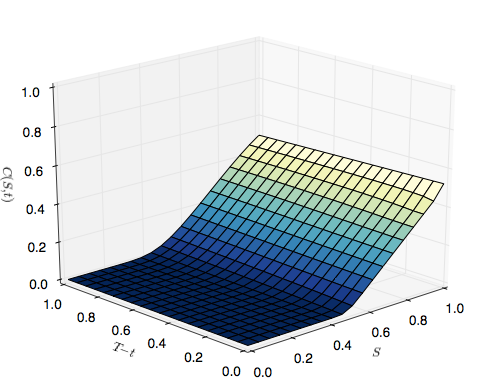
European vanilla call price surface, $C(S,t)$
Note that at $T-t = 0.0$, when the option expires, the profile follows that for a vanilla call option pay-off. This is a non-smooth piecewise linear pay-off function, with a turning point at the point at which spot equals strike, i.e. $S=K$. As the option is "marched back in time" via the FDM solver, the profile "smooths out" (see the smoothed region around $S=K$ at $T-t=1.0$). This is exactly the same behaviour as in a forward heat equation, where heat diffuses from an initial profile to a smoother profile.
The next articles will concentrate on more sophisticated ways of solving the equation, specifically via the semi-implicit Crank-Nicolson techniques as well as more recent methods.


