Article updated April 2022 for Python 3.8
Over the last few years we have spent a good deal of time on QuantStart considering option price models, time series analysis and quantitative trading. It has become clear to me that many of you are interested in learning about the modern mathematical techniques that underpin not only quantitative finance and algorithmic trading, but also the newly emerging fields of data science and statistical machine learning.
Quantitative skills are now in high demand not only in the financial sector but also at consumer technology startups, as well as larger data-driven firms. Hence we are going to expand the topics discussed on QuantStart to include not only modern financial techniques, but also statistical learning as applied to other areas, in order to broaden your career prospects if you are quantitatively focused.
In order to begin discussing the modern techniques, we must first gain a solid understanding in the underlying mathematics and statistics that underpins these models. One of the key modern areas is that of Bayesian Statistics. We have not yet discussed Bayesian methods in any great detail on the site. This article has been written to help you understand the "philosophy" of the Bayesian approach, how it compares to the traditional/classical frequentist approach to statistics and the potential applications in both quantitative finance and data science.
In the article we will:
- Define Bayesian statistics (or Bayesian inference)
- Compare Classical ("Frequentist") statistics and Bayesian statistics
- Derive the famous Bayes' rule, an essential tool for Bayesian inference
- Interpret and apply Bayes' rule for carrying out Bayesian inference
- Carry out a concrete probability coin-flip example of Bayesian inference
What is Bayesian Statistics?
Bayesian statistics is a particular approach to applying probability to statistical problems. It provides us with mathematical tools to update our beliefs about random events in light of seeing new data or evidence about those events.
In particular Bayesian inference interprets probability as a measure of believability or confidence that an individual may possess about the occurance of a particular event.
We may have a prior belief about an event, but our beliefs are likely to change when new evidence is brought to light. Bayesian statistics gives us a solid mathematical means of incorporating our prior beliefs, and evidence, to produce new posterior beliefs.
Bayesian statistics provides us with mathematical tools to rationally update our subjective beliefs in light of new data or evidence.
This is in contrast to another form of statistical inference, known as classical or frequentist statistics, which assumes that probabilities are the frequency of particular random events occuring in a long run of repeated trials.
For example, as we roll a fair (i.e. unweighted) six-sided die repeatedly, we would see that each number on the die tends to come up 1/6 of the time.
Frequentist statistics assumes that probabilities are the long-run frequency of random events in repeated trials.
When carrying out statistical inference, that is, inferring statistical information from probabilistic systems, the two approaches - frequentist and Bayesian - have very different philosophies.
Frequentist statistics tries to eliminate uncertainty by providing estimates. Bayesian statistics tries to preserve and refine uncertainty by adjusting individual beliefs in light of new evidence.
Frequentist vs Bayesian Examples
In order to make clear the distinction between the two differing statistical philosophies, we will consider two examples of probabilistic systems:
- Coin flips - What is the probability of an unfair coin coming up heads?
- Election of a particular candidate for UK Prime Minister - What is the probability of seeing an individual candidate winning, who has not stood before?
The following table describes the alternative philosophies of the frequentist and Bayesian approaches:
| Example | Frequentist Interpretation | Bayesian Interpretation |
|---|---|---|
| Unfair Coin Flip | The probability of seeing a head when the unfair coin is flipped is the long-run relative frequency of seeing a head when repeated flips of the coin are carried out. That is, as we carry out more coin flips the number of heads obtained as a proportion of the total flips tends to the "true" or "physical" probability of the coin coming up as heads. In particular the individual running the experiment does not incorporate their own beliefs about the fairness of other coins. | Prior to any flips of the coin an individual may believe that the coin is fair. After a few flips the coin continually comes up heads. Thus the prior belief about fairness of the coin is modified to account for the fact that three heads have come up in a row and thus the coin might not be fair. After 500 flips, with 400 heads, the individual believes that the coin is very unlikely to be fair. The posterior belief is heavily modified from the prior belief of a fair coin. |
| Election of Candidate | The candidate only ever stands once for this particular election and so we cannot perform "repeated trials". In a frequentist setting we construct "virtual" trials of the election process. The probability of the candidate winning is defined as the relative frequency of the candidate winning in the "virtual" trials as a fraction of all trials. | An individual has a prior belief of a candidate's chances of winning an election and their confidence can be quantified as a probability. However another individual could also have a separate differing prior belief about the same candidate's chances. As new data arrives, both beliefs are (rationally) updated by the Bayesian procedure. |
Thus in the Bayesian interpretation a probability is a summary of an individual's opinion. A key point is that different (intelligent) individuals can have different opinions (and thus different prior beliefs), since they have differing access to data and ways of interpreting it. However, as both of these individuals come across new data that they both have access to their (potentially differing) prior beliefs will lead to posterior beliefs that will begin converging towards each other under the rational updating procedure of Bayesian inference.
In the Bayesian framework an individual would apply a probability of 0 when they have no confidence in an event occuring, while they would apply a probability of 1 when they are absolutely certain of an event occuring. A probability assigned between 0 and 1 allows weighted confidence in other potential outcomes.
In order to carry out Bayesian inference, we need to utilise a famous theorem in probability known as Bayes' rule and interpret it in the correct fashion. In the following box, we derive Bayes' rule using the definition of conditional probability. However, it isn't essential to follow the derivation in order to use Bayesian methods, so feel free to skip the box if you wish to jump straight into learning how to use Bayes' rule.
Deriving Bayes' Rule
We begin by considering the definition of conditional probability, which gives us a rule for determining the probability of an event $A$, given the occurance of another event $B$. An example question in this vein might be "What is the probability of rain occuring given that there are clouds in the sky?"
The mathematical definition of conditional probability is as follows:
\begin{eqnarray} P(A|B) = \frac{P(A \cap B)}{P(B)} \end{eqnarray}This simply states that the probability of $A$ occuring given that $B$ has occured is equal to the probability that they have both occured, relative to the probability that $B$ has occured.
Or in the language of the example above: The probability of rain given that we have seen clouds is equal to the probability of rain and clouds occuring together, relative to the probability of seeing clouds at all.
If we multiply both sides of this equation by $P(B)$ we get:
\begin{eqnarray} P(B) P(A|B) = P(A \cap B) \end{eqnarray}But, we can simply make the same statement about $P(B|A)$, which is akin to asking "What is the probability of seeing clouds, given that it is raining?":
\begin{eqnarray} P(B|A) = \frac{P(B \cap A)}{P(A)} \end{eqnarray}Note that $P(A \cap B) = P(B \cap A)$ and so by substituting the above and multiplying by $P(A)$, we get:
\begin{eqnarray} P(A) P(B|A) = P(A \cap B) \end{eqnarray}We are now able to set the two expressions for $P(A \cap B)$ equal to each other:
\begin{eqnarray} P(B) P(A|B) = P(A) P(B|A) \end{eqnarray}If we now divide both sides by $P(B)$ we arrive at the celebrated Bayes' rule:
\begin{eqnarray} P(A|B) = \frac{P(B|A) P(A)}{P(B)} \end{eqnarray}However, it will be helpful for later usage of Bayes' rule to modify the denominator, $P(B)$ on the right hand side of the above relation to be written in terms of $P(B|A)$. We can actually write:
\begin{eqnarray} P(B) = \sum_{a \in A} P(B \cap A) \end{eqnarray}This is possible because the events $A$ are an exhaustive partition of the sample space.
So that by substituting the defintion of conditional probability we get:
\begin{eqnarray} P(B) = \sum_{a \in A} P(B \cap A) = \sum_{a \in A} P(B|A) P(A) \end{eqnarray}Finally, we can substitute this into Bayes' rule from above to obtain an alternative version of Bayes' rule, which is used heavily in Bayesian inference:
\begin{eqnarray} P(A|B) = \frac{P(B|A) P(A)}{\sum_{a \in A} P(B|A) P(A)} \end{eqnarray}Now that we have derived Bayes' rule we are able to apply it to statistical inference.
Applying Bayes' Rule for Bayesian Inference
As we stated at the start of this article the basic idea of Bayesian inference is to continually update our prior beliefs about events as new evidence is presented. This is a very natural way to think about probabilistic events. As more and more evidence is accumulated our prior beliefs are steadily "washed out" by any new data.
Consider a (rather nonsensical) prior belief that the Moon is going to collide with the Earth. For every night that passes, the application of Bayesian inference will tend to correct our prior belief to a posterior belief that the Moon is less and less likely to collide with the Earth, since it remains in orbit.
In order to demonstrate a concrete numerical example of Bayesian inference it is necessary to introduce some new notation.
Firstly, we need to consider the concept of parameters and models. A parameter could be the weighting of an unfair coin, which we could label as $\theta$. Thus $\theta = P(H)$ would describe the probability distribution of our beliefs that the coin will come up as heads when flipped. The model is the actual means of encoding this flip mathematically. In this instance, the coin flip can be modelled as a Bernoulli trial.
Bernoulli Trial
A Bernoulli trial is a random experiment with only two outcomes, usually labelled as "success" or "failure", in which the probability of the success is exactly the same every time the trial is carried out. The probability of the success is given by $\theta$, which is a number between 0 and 1. Thus $\theta \in [0,1]$.
Over the course of carrying out some coin flip experiments (repeated Bernoulli trials) we will generate some data, $D$, about heads or tails.
A natural example question to ask is "What is the probability of seeing 3 heads in 8 flips (8 Bernoulli trials), given a fair coin ($\theta=0.5$)?".
A model helps us to ascertain the probability of seeing this data, $D$, given a value of the parameter $\theta$. The probability of seeing data $D$ under a particular value of $\theta$ is given by the following notation: $P(D|\theta)$.
However, if you consider it for a moment, we are actually interested in the alternative question - "What is the probability that the coin is fair (or unfair), given that I have seen a particular sequence of heads and tails?".
Thus we are interested in the probability distribution which reflects our belief about different possible values of $\theta$, given that we have observed some data $D$. This is denoted by $P(\theta|D)$. Notice that this is the converse of $P(D|\theta)$. So how do we get between these two probabilities? It turns out that Bayes' rule is the link that allows us to go between the two situations.
Bayes' Rule for Bayesian Inference
\begin{eqnarray} P(\theta|D) = P(D|\theta) \; P(\theta) \; / \; P(D) \end{eqnarray}Where:
- $P(\theta)$ is the prior. This is the strength in our belief of $\theta$ without considering the evidence $D$. Our prior view on the probability of how fair the coin is.
- $P(\theta|D)$ is the posterior. This is the (refined) strength of our belief of $\theta$ once the evidence $D$ has been taken into account. After seeing 4 heads out of 8 flips, say, this is our updated view on the fairness of the coin.
- $P(D|\theta)$ is the likelihood. This is the probability of seeing the data $D$ as generated by a model with parameter $\theta$. If we knew the coin was fair, this tells us the probability of seeing a number of heads in a particular number of flips.
- $P(D)$ is the evidence. This is the probability of the data as determined by summing (or integrating) across all possible values of $\theta$, weighted by how strongly we believe in those particular values of $\theta$. If we had multiple views of what the fairness of the coin is (but didn't know for sure), then this tells us the probability of seeing a certain sequence of flips for all possibilities of our belief in the coin's fairness.
The entire goal of Bayesian inference is to provide us with a rational and mathematically sound procedure for incorporating our prior beliefs, with any evidence at hand, in order to produce an updated posterior belief. What makes it such a valuable technique is that posterior beliefs can themselves be used as prior beliefs under the generation of new data. Hence Bayesian inference allows us to continually adjust our beliefs under new data by repeatedly applying Bayes' rule.
There was a lot of theory to take in within the previous two sections, so I'm now going to provide a concrete example using the age-old tool of statisticians: the coin-flip.
Coin-Flipping Example
In this example we are going to consider multiple coin-flips of a coin with unknown fairness. We will use Bayesian inference to update our beliefs on the fairness of the coin as more data (i.e. more coin flips) becomes available. The coin will actually be fair, but we won't learn this until the trials are carried out. At the start we have no prior belief on the fairness of the coin, that is, we can say that any level of fairness is equally likely.
In statistical language we are going to perform $N$ repeated Bernoulli trials with $\theta = 0.5$. We will use a uniform distribution as a means of characterising our prior belief that we are unsure about the fairness. This states that we consider each level of fairness (or each value of $\theta$) to be equally likely.
We are going to use a Bayesian updating procedure to go from our prior beliefs to posterior beliefs as we observe new coin flips. This is carried out using a particularly mathematically succinct procedure using conjugate priors. We won't go into any detail on conjugate priors within this article, as it will form the basis of the next article on Bayesian inference. It will however provide us with the means of explaining how the coin flip example is carried out in practice.
The uniform distribution is actually a more specific case of another probability distribution, known as a Beta distribution. Conveniently, under the binomial model, if we use a Beta distribution for our prior beliefs it leads to a Beta distribution for our posterior beliefs. This is an extremely useful mathematical result, as Beta distributions are quite flexible in modelling beliefs. However, I don't want to dwell on the details of this too much here, since we will discuss it in the next article. At this stage, it just allows us to easily create some visualisations below that emphasises the Bayesian procedure!
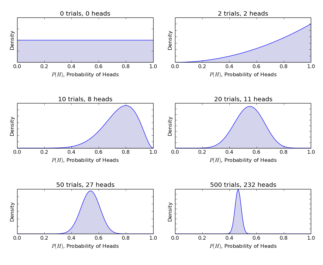
In the following figure we can see 6 particular points at which we have carried out a number of Bernoulli trials (coin flips). In the first sub-plot we have carried out no trials and hence our probability density function (in this case our prior density) is the uniform distribution. It states that we have equal belief in all values of $\theta$ representing the fairness of the coin.
The next panel shows 2 trials carried out and they both come up heads. Our Bayesian procedure using the conjugate Beta distributions now allows us to update to a posterior density. Notice how the weight of the density is now shifted to the right hand side of the chart. This indicates that our prior belief of equal likelihood of fairness of the coin, coupled with 2 new data points, leads us to believe that the coin is more likely to be unfair (biased towards heads) than it is tails.
The following two panels show 10 and 20 trials respectively. Notice that even though we have seen 2 tails in 10 trials we are still of the belief that the coin is likely to be unfair and biased towards heads. After 20 trials, we have seen a few more tails appear. The density of the probability has now shifted closer to $\theta=P(H)=0.5$. Hence we are now starting to believe that the coin is possibly fair.
After 50 and 500 trials respectively, we are now beginning to believe that the fairness of the coin is very likely to be around $\theta=0.5$. This is indicated by the shrinking width of the probability density, which is now clustered tightly around $\theta=0.46$ in the final panel. Were we to carry out another 500 trials (since the coin is actually fair) we would see this probability density become even tighter and centred closer to $\theta=0.5$.
Thus it can be seen that Bayesian inference gives us a rational procedure to go from an uncertain situation with limited information to a more certain situation with significant amounts of data. In the next article we will discuss the notion of conjugate priors in more depth, which heavily simplify the mathematics of carrying out Bayesian inference in this example.
For completeness, I've provided the Python code (heavily commented) for producing this plot. It makes use of SciPy's statistics model, in particular, the Beta distribution:
import numpy as np
from scipy import stats
from matplotlib import pyplot as plt


if __name__ == "__main__":
    # Create a list of the number of coin tosses ("Bernoulli trials")
    number_of_trials = [0, 2, 10, 20, 50, 500]

    # Conduct 500 coin tosses and output into a list of 0s and 1s
    # where 0 represents a tail and 1 represents a head
    data = stats.bernoulli.rvs(0.5, size=number_of_trials[-1])

    # Discretise the x-axis into 100 separate plotting points
    x = np.linspace(0, 1, 100)

    # Loops over the number_of_trials list to continually add
    # more coin toss data. For each new set of data, we update
    # our (current) prior belief to be a new posterior. This is
    # carried out using what is known as the Beta-Binomial model.
    # For the time being, we won't worry about this too much. It
    # will be the subject of a later article!
    for i, N in enumerate(number_of_trials):
        # Accumulate the total number of heads for this
        # particular Bayesian update
        heads = data[:N].sum()

        # Create an axes subplot for each update
        ax = plt.subplot(int(len(number_of_trials) / 2), 2, i + 1)
        ax.set_title("%s trials, %s heads" % (N, heads))

        # Add labels to both axes and hide labels on y-axis
        plt.xlabel("$P(H)$, Probability of Heads")
        plt.ylabel("Density")
        if i == 0:
            plt.ylim([0.0, 2.0])
        plt.setp(ax.get_yticklabels(), visible=False)

        # Create and plot a  Beta distribution to represent the
        # posterior belief in fairness of the coin.
        y = stats.beta.pdf(x, 1 + heads, 1 + N - heads)
        plt.plot(x, y, label="observe %d tosses,\n %d heads" % (N, heads))
        plt.fill_between(x, 0, y, color="#aaaadd", alpha=0.5)

    # Expand plot to cover full width/height and show it
    plt.tight_layout()
    plt.show()
I'd like to give special thanks to my good friend Jonathan Bartlett, who runs TheStatsGeek.com, for reading drafts of this article and for providing helpful advice on interpretation and corrections. Thanks Jon!