Recently on QuantStart we've discussed machine learning, forecasting, backtesting design and backtesting implementation. We are now going to combine all of these previous tools to backtest a financial forecasting algorithm for the S&P500 US stock market index by trading on the SPY ETF.
This article will build heavily on the software we have already developed in the articles mentioned above, including the object-oriented backtesting engine and the forecasting signal generator. The nature of object-oriented programming means that the code we write subsequently can be kept short as the "heavy lifting" is carried out on classes we have already developed.
Mature Python libraries such as matplotlib, pandas and scikit-learn also reduce the necessity to write boilerplate code or come up with our own implementations of well known algorithms.
The Forecasting Strategy
The forecasting strategy itself is based on a machine learning technique known as a quadratic discriminant analyser, which is closely related to a linear discriminant analyser. Both of these models are described in detail within the article on forecasting of financial time series.
The forecaster uses the previous two daily returns as a set of factors to predict todays direction of the stock market. If the probability of the day being "up" exceeds 50%, the strategy purchases 500 shares of the SPY ETF and sells it at the end of the day. if the probability of a down day exceeds 50%, the strategy sells 500 shares of the SPY ETF and then buys back at the close. Thus it is our first example of an intraday trading strategy.
Note that this is not a particularly realistic trading strategy! We are unlikely to ever achieve an opening or closing price due to many factors such as excessive opening volatility, order routing by the brokerage and potential liquidity issues around the open/close. In addition we have not included transaction costs. These would likely be a substantial percentage of the returns as there is a round-trip trade carried out every day. Thus our forecaster needs to be relatively accurate at predicting daily returns, otherwise transaction costs will eat all of our trading returns.
Implementation
As with the other Python/pandas related tutorials I have used the following libraries:
- Python - 2.7.3
- NumPy - 1.8.0
- pandas - 0.12.0
- matplotlib - 1.1.0
- scikit-learn - 0.14.1
The implementation of snp_forecast.py below requires backtest.py from this previous tutorial. In addition forecast.py (which mainly contains the function create_lagged_series) is created from this previous tutorial. The first step is to import the necessary modules and objects:
# snp_forecast.py

import datetime
import matplotlib.pyplot as plt
import numpy as np
import pandas as pd
import sklearn

from pandas.io.data import DataReader
from sklearn.qda import QDA

from backtest import Strategy, Portfolio
from forecast import create_lagged_series
Once all of the relevant libraries and modules have been included it is time to subclass the Strategy abstract base class, as we have carried out in previous tutorials. SNPForecastingStrategy is designed to fit a Quadratic Discriminant Analyser to the S&P500 stock index as a means of predicting its future value. The fitting of the model is carried out in the fit_model method below, while the actual signals are generated from the generate_signals method. This matches the interface of a Strategy class.
The details of how a quadratic discriminant analyser works, as well as the Python implementation below, is described in detail in the previous article on forecasting of financial time series. The comments in the source code below discuss extensively what the program is doing:
# snp_forecast.py

class SNPForecastingStrategy(Strategy):
    """
    Requires:
    symbol - A stock symbol on which to form a strategy on.
    bars - A DataFrame of bars for the above symbol."""

    def __init__(self, symbol, bars):
        self.symbol = symbol
        self.bars = bars
        self.create_periods()
        self.fit_model()

    def create_periods(self):
        """Create training/test periods."""
        self.start_train = datetime.datetime(2001,1,10)
        self.start_test = datetime.datetime(2005,1,1)
        self.end_period = datetime.datetime(2005,12,31)

    def fit_model(self):
        """Fits a Quadratic Discriminant Analyser to the
        US stock market index (^GPSC in Yahoo)."""
        # Create a lagged series of the S&P500 US stock market index
        snpret = create_lagged_series(self.symbol, self.start_train,
                                      self.end_period, lags=5)

        # Use the prior two days of returns as
        # predictor values, with direction as the response
        X = snpret[["Lag1","Lag2"]]
        y = snpret["Direction"]

        # Create training and test sets
        X_train = X[X.index < self.start_test]
        y_train = y[y.index < self.start_test]

        # Create the predicting factors for use
        # in direction forecasting
        self.predictors = X[X.index >= self.start_test]

        # Create the Quadratic Discriminant Analysis model
        # and the forecasting strategy
        self.model = QDA()
        self.model.fit(X_train, y_train)

    def generate_signals(self):
        """Returns the DataFrame of symbols containing the signals
        to go long, short or hold (1, -1 or 0)."""
        signals = pd.DataFrame(index=self.bars.index)
        signals['signal'] = 0.0

        # Predict the subsequent period with the QDA model
        signals['signal'] = self.model.predict(self.predictors)

        # Remove the first five signal entries to eliminate
        # NaN issues with the signals DataFrame
        signals['signal'][0:5] = 0.0
        signals['positions'] = signals['signal'].diff()

        return signals
Now that the forecasting engine has produced the signals, we can create a MarketIntradayPortfolio. This portfolio object differs from the example given in the Moving Average Crossover backtest article as it carries out trading on an intraday basis.
The portfolio is designed to "go long" (buy) 500 shares of SPY at the opening price if the signal states that an up-day will occur and then sell at the close. Conversely, the portfolio is designed "go short" (sell) 500 shares of SPY if the signal states that a down-day will occur and subsequently close out at the closing price.
To achieve this the price difference between the market open and market close prices are determined every day, leading to a calculation of daily profit on the 500 shares bought or sold. This then leads naturally to an equity curve by cumulatively summing up the profit/loss for each day. It also has the benefit of allowing us to calculate profit/loss statistics for each day.
Here is the listing for the MarketIntradayPortfolio:
# snp_forecast.py

class MarketIntradayPortfolio(Portfolio):
    """Buys or sells 500 shares of an asset at the opening price of
    every bar, depending upon the direction of the forecast, closing
    out the trade at the close of the bar.

    Requires:
    symbol - A stock symbol which forms the basis of the portfolio.
    bars - A DataFrame of bars for a symbol set.
    signals - A pandas DataFrame of signals (1, 0, -1) for each symbol.
    initial_capital - The amount in cash at the start of the portfolio."""

    def __init__(self, symbol, bars, signals, initial_capital=100000.0):
        self.symbol = symbol
        self.bars = bars
        self.signals = signals
        self.initial_capital = float(initial_capital)
        self.positions = self.generate_positions()

    def generate_positions(self):
        """Generate the positions DataFrame, based on the signals
        provided by the 'signals' DataFrame."""
        positions = pd.DataFrame(index=self.signals.index).fillna(0.0)

        # Long or short 500 shares of SPY based on
        # directional signal every day
        positions[self.symbol] = 500*self.signals['signal']
        return positions

    def backtest_portfolio(self):
        """Backtest the portfolio and return a DataFrame containing
        the equity curve and the percentage returns."""

        # Set the portfolio object to have the same time period
        # as the positions DataFrame
        portfolio = pd.DataFrame(index=self.positions.index)
        pos_diff = self.positions.diff()

        # Work out the intraday profit of the difference
        # in open and closing prices and then determine
        # the daily profit by longing if an up day is predicted
        # and shorting if a down day is predicted
        portfolio['price_diff'] = self.bars['Close']-self.bars['Open']
        portfolio['price_diff'][0:5] = 0.0
        portfolio['profit'] = self.positions[self.symbol] * portfolio['price_diff']

        # Generate the equity curve and percentage returns
        portfolio['total'] = self.initial_capital + portfolio['profit'].cumsum()
        portfolio['returns'] = portfolio['total'].pct_change()
        return portfolio
The final step is to tie the Strategy and Portfolio objects together with a __main__ function. The function obtains the data for the SPY instrument and then creates the signal generating strategy on the S&P500 index itself. This is provided by the ^GSPC ticker. Then a MarketIntradayPortfolio is generated with an initial capital of 100,000 USD (as in previous tutorials). Finally, the returns are calculated and the equity curve is plotted.
Note how little code is required at this stage because all of the heavy computation is carried out in the Strategy and Portfolio subclasses. This makes it extremely straightforward to create new trading strategies and test them rapidly for use in the "strategy pipeline".
if __name__ == "__main__":
    start_test = datetime.datetime(2005,1,1)
    end_period = datetime.datetime(2005,12,31)

    # Obtain the bars for SPY ETF which tracks the S&P500 index
    bars = DataReader("SPY", "yahoo", start_test, end_period)

    # Create the S&P500 forecasting strategy
    snpf = SNPForecastingStrategy("^GSPC", bars)
    signals = snpf.generate_signals()

    # Create the portfolio based on the forecaster
    portfolio = MarketIntradayPortfolio("SPY", bars, signals,
                                        initial_capital=100000.0)
    returns = portfolio.backtest_portfolio()

    # Plot results
    fig = plt.figure()
    fig.patch.set_facecolor('white')

    # Plot the price of the SPY ETF
    ax1 = fig.add_subplot(211,  ylabel='SPY ETF price in $')
    bars['Close'].plot(ax=ax1, color='r', lw=2.)

    # Plot the equity curve
    ax2 = fig.add_subplot(212, ylabel='Portfolio value in $')
    returns['total'].plot(ax=ax2, lw=2.)

    fig.show()
The output of the program is given below. In this period the stock market returned 4% (assuming a fully invested buy and hold strategy), while the algorithm itself also returned 4%. Note that transaction costs (such as commission fees) have not been added to this backtesting system. Since the strategy carries out a round-trip trade once per day, these fees are likely to significantly curtail the returns.
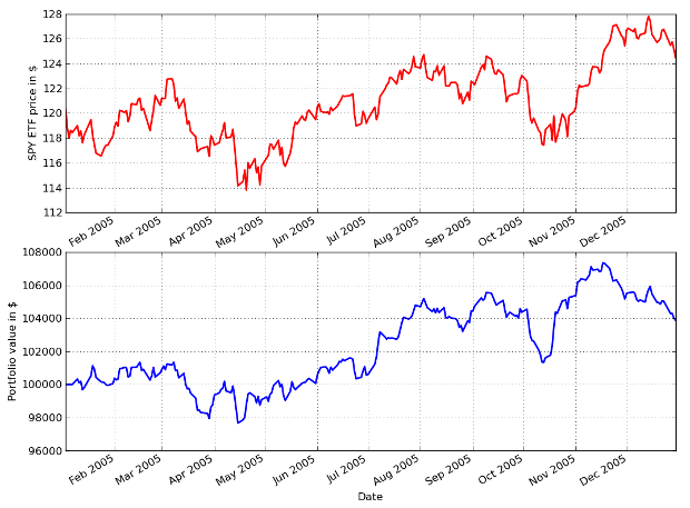
S&P500 Forecasting Strategy Performance from 2005-01-01 to 2006-12-31
In subsequent articles we will add realistic transaction costs, utilise additional forecasting engines, determine performance metrics and provide portfolio optimisation tools.


