In Part 1 we considered the Autoregressive model of order p, also known as the AR(p) model. We introduced it as an extension of the random walk model in an attempt to explain additional serial correlation in financial time series.
Ultimately we realised that it was not sufficiently flexible to truly capture all of the autocorrelation in the closing prices of Amazon Inc. (AMZN) and the S&P500 US Equity Index. The primary reason for this is that both of these assets are conditionally heteroskedastic, which means that they are non-stationary and have periods of "varying variance" or volatility clustering, which is not taken into account by the AR(p) model.
In future articles we will eventually build up to the Autoregressive Integrated Moving Average (ARIMA) models, as well as the conditionally heteroskedastic models of the ARCH and GARCH families. These models will provide us with our first realistic attempts at forecasting asset prices.
In this article, however, we are going to introduce the Moving Average of order q model, known as MA(q). This is a component of the more general ARMA model and as such we need to understand it before moving further.
I highly recommend you read the previous articles in the Time Series Analysis collection if you have not done so. They can all be found here.
Moving Average (MA) Models of order q
Rationale
A Moving Average model is similar to an Autoregressive model, except that instead of being a linear combination of past time series values, it is a linear combination of the past white noise terms.
Intuitively, this means that the MA model sees such random white noise "shocks" directly at each current value of the model. This is in contrast to an AR(p) model, where the white noise "shocks" are only seen indirectly, via regression onto previous terms of the series.
A key difference is that the MA model will only ever see the last $q$ shocks for any particular MA(q) model, whereas the AR(p) model will take all prior shocks into account, albeit in a decreasingly weak manner.
Definition
Mathematically, the MA(q) is a linear regression model and is similarly structured to AR(p):
Moving Average Model of order q
A time series model, $\{ x_t \}$, is a moving average model of order $q$, MA(q), if:
\begin{eqnarray} x_t = w_t + \beta_1 w_{t-1} + \ldots + \beta_q w_{t-q} \end{eqnarray}Where $\{ w_t \}$ is white noise with $E(w_t) = 0$ and variance $\sigma^2$.
If we consider the Backward Shift Operator, ${\bf B}$ (see a previous article) then we can rewrite the above as a function $\phi$ of ${\bf B}$:
\begin{eqnarray} x_t = (1 + \beta_1 {\bf B} + \beta_2 {\bf B}^2 + \ldots + \beta_q {\bf B}^q) w_t = \phi_q ({\bf B}) w_t \end{eqnarray}We will make use of the $\phi$ function in later articles.
Second Order Properties
As with AR(p) the mean of a MA(q) process is zero. This is easy to see as the mean is simply a sum of means of white noise terms, which are all themselves zero.
\begin{eqnarray} \text{Mean:} \enspace \mu_x = E(x_t) = \sum^{q}_{i=0} E(w_i) = 0 \end{eqnarray} \begin{eqnarray} \text{Var:} \enspace \sigma^2_w (1 + \beta^2_1 + \ldots + \beta^2_q) \end{eqnarray} $$\text{ACF:} \enspace \rho_k = \left\{\begin{aligned} &1 && \text{if} \enspace k = 0 \\ &\sum^{q-k}_{i=0} \beta_i \beta_{i+k} / \sum^q_{i=0} \beta^2_i && \text{if} \enspace k = 1, \ldots, q \\ &0 && \text{if} \enspace k > q \end{aligned} \right.$$Where $\beta_0 = 1$.
We're now going to generate some simulated data and use it to create correlograms. This will make the above formula for $\rho_k$ somewhat more concrete.
Simulations and Correlograms
MA(1)
Let's start with a MA(1) process. If we set $\beta_1 = 0.6$ we obtain the following model:
\begin{eqnarray} x_t = w_t + 0.6 w_{t-1} \end{eqnarray}As with the AR(p) models in the previous article we can use R to simulate such a series and then plot the correlogram. Since we've had a lot of practice in the previous Time Series Analysis article series of carrying out plots, I will write the R code in full, rather than splitting it up:
> set.seed(1)
> x <- w <- rnorm(100)
> for (t in 2:100) x[t] <- w[t] + 0.6*w[t-1]
> layout(1:2)
> plot(x, type="l")
> acf(x)
The output is as follows:
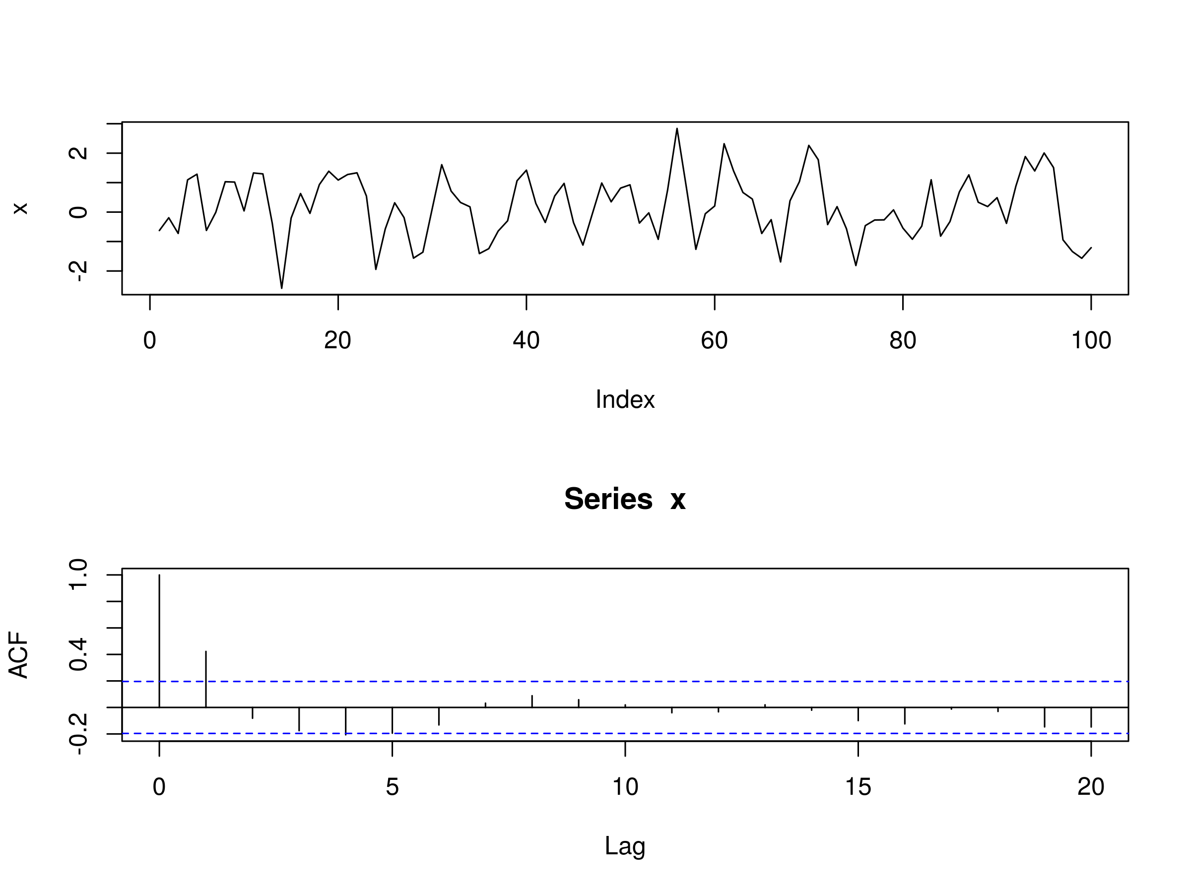 Realisation of MA(1) Model, with $\beta_1 = 0.6$ and Associated Correlogram
As we saw above in the formula for $\rho_k$, for $k > q$, all autocorrelations should be zero. Since $q = 1$, we should see a significant peak at $k=1$ and then insignificant peaks subsequent to that. However, due to sampling bias we should expect to see 5% (marginally) significant peaks on a sample autocorrelation plot.
This is precisely what the correlogram shows us in this case. We have a significant peak at $k=1$ and then insignificant peaks for $k > 1$, except at $k=4$ where we have a marginally significant peak.
In fact, this is a useful way of seeing whether an MA(q) model is appropriate. By taking a look at the correlogram of a particular series we can see how many sequential non-zero lags exist. If $q$ such lags exist then we can legitimately attempt to fit a MA(q) model to a particular series.
Since we have evidence from our simulated data of a MA(1) process, we're now going to try and fit a MA(1) model to our simulated data. Unfortunately, there isn't an equivalent ma command to the autoregressive model ar command in R.
Instead, we must use the more general arima command and set the autoregressive and integrated components to zero. We do this by creating a 3-vector and setting the first two components (the autogressive and integrated parameters, respectively) to zero:
> x.ma <- arima(x, order=c(0, 0, 1))
> x.ma
Call:
arima(x = x, order = c(0, 0, 1))

Coefficients:
         ma1  intercept
      0.6023     0.1681
s.e.  0.0827     0.1424

sigma^2 estimated as 0.7958:  log likelihood = -130.7,  aic = 267.39
We receive some useful output from the arima command. Firstly, we can see that the parameter has been estimated as $\hat{\beta_1} = 0.602$, which is very close to the true value of $\beta_1 = 0.6$. Secondly, the standard errors are already calculated for us, making it straightforward to calculate confidence intervals. Thirdly, we receive an estimated variance, log-likelihood and Akaike Information Criterion (necessary for model comparison).
The major difference between arima and ar is that arima estimates an intercept term because it does not subtract the mean value of the series. Hence we need to be careful when carrying out predictions using the arima command. We'll return to this point later.
As a quick check we're going to calculate confidence intervals for $\hat{\beta_1}$:
> 0.6023 + c(-1.96, 1.96)*0.0827
0.440208 0.764392
We can see that the 95% confidence interval contains the true parameter value of $\beta_1 = 0.6$ and so we can judge the model a good fit. Obviously this should be expected since we simulated the data in the first place!
How do things change if we modify the sign of $\beta_1$ to -0.6? Let's perform the same analysis:
> set.seed(1)
> x <- w <- rnorm(100)
> for (t in 2:100) x[t] <- w[t] - 0.6*w[t-1]
> layout(1:2)
> plot(x, type="l")
> acf(x)
The output is as follows:
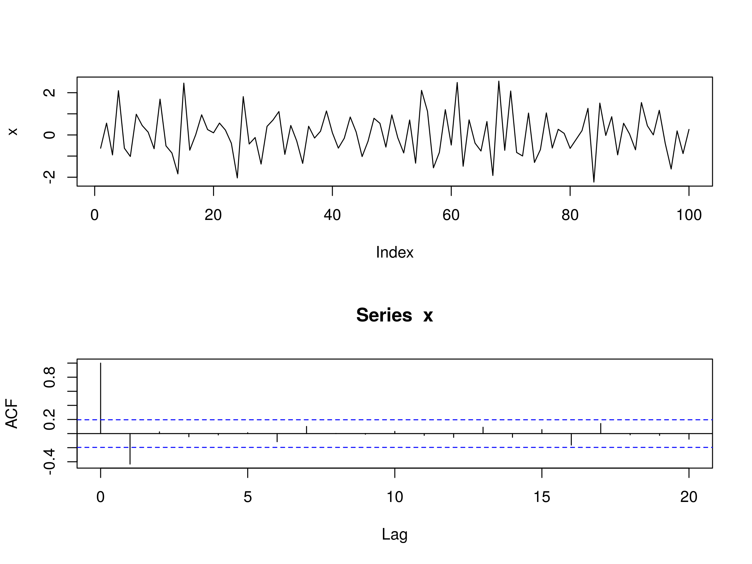 Realisation of MA(1) Model, with $\beta_1 = -0.6$ and Associated Correlogram
We can see that at $k=1$ we have a significant peak in the correlogram, except that it shows negative correlation, as we'd expect from a MA(1) model with negative first coefficient. Once again all peaks beyond $k=1$ are insignificant. Let's fit a MA(1) model and estimate the parameter:
> x.ma <- arima(x, order=c(0, 0, 1))
> x.ma
Call:
arima(x = x, order = c(0, 0, 1))

Coefficients:
          ma1  intercept
      -0.7298     0.0486
s.e.   0.1008     0.0246

sigma^2 estimated as 0.7841:  log likelihood = -130.11,  aic = 266.23
$\hat{\beta_1} = -0.730$, which is a small underestimate of $\beta_1 = -0.6$. Finally, let's calculate the confidence interval:
> -0.730 + c(-1.96, 1.96)*0.1008
-0.927568 -0.532432
We can see that the true parameter value of $\beta_1=-0.6$ is contained within the 95% confidence interval, providing us with evidence of a good model fit.
MA(3)
Let's run through the same procedure for a MA(3) process. This time we should expect significant peaks at $k \in \{1,2,3 \}$, and insignificant peaks for $k > 3$.
We are going to use the following coefficients: $\beta_1 = 0.6$, $\beta_2 = 0.4$ and $\beta_3 = 0.2$. Let's simulate a MA(3) process from this model. I've increased the number of random samples to 1000 in this simulation, which makes it easier to see the true autocorrelation structure, at the expense of making the original series harder to interpret:
> set.seed(3)
> x <- w <- rnorm(1000)
> for (t in 4:1000) x[t] <- w[t] + 0.6*w[t-1] + 0.4*w[t-2] + 0.3*w[t-3]
> layout(1:2)
> plot(x, type="l")
> acf(x)
The output is as follows:
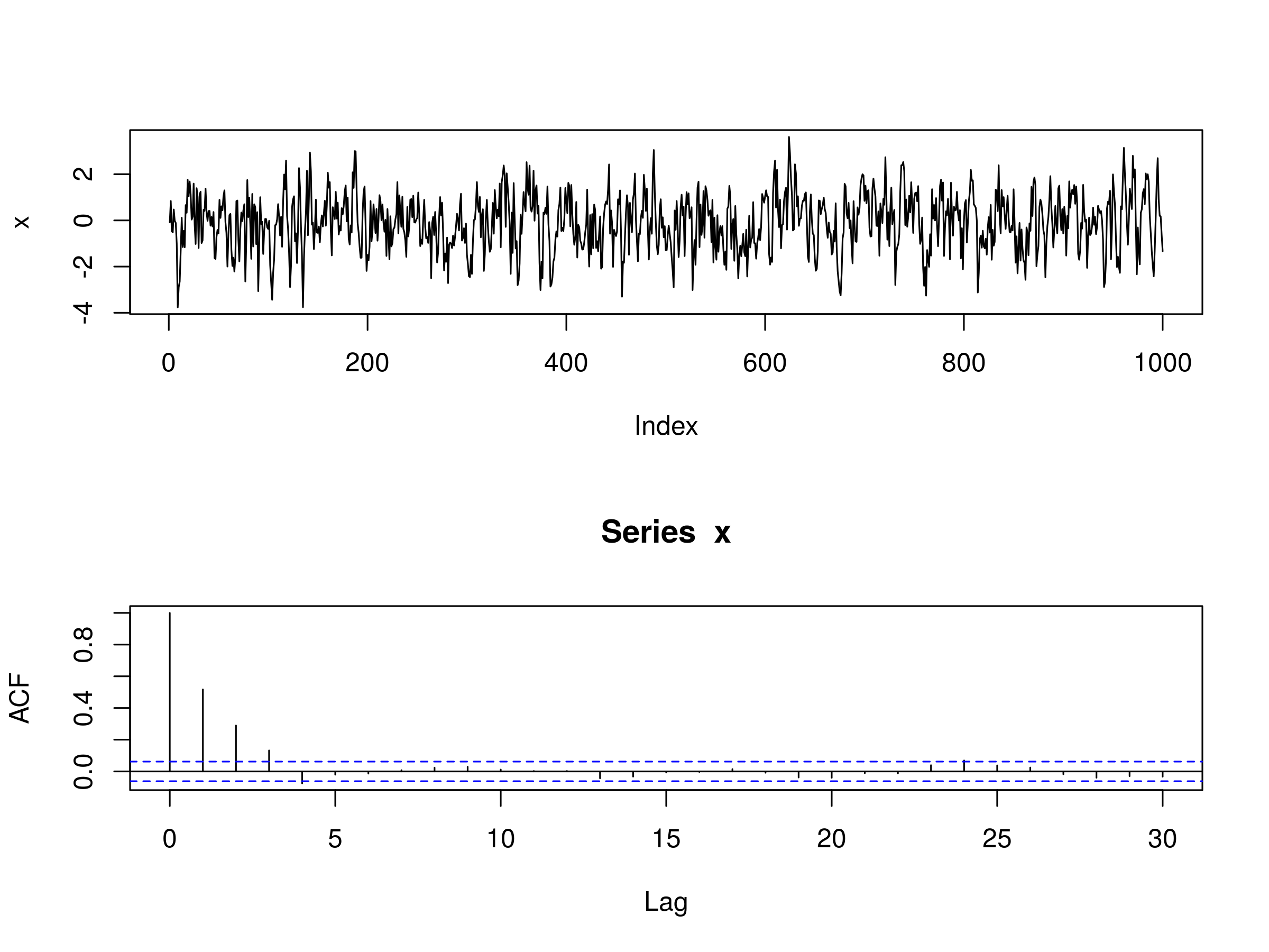 Realisation of MA(3) Model and Associated Correlogram
As expected the first three peaks are significant. However, so is the fourth. But we can legitimately suggest that this may be due to sampling bias as we expect to see 5% of the peaks being significant beyond $k=q$.
Let's now fit a MA(3) model to the data to try and estimate parameters:
> x.ma <- arima(x, order=c(0, 0, 3))
> x.ma
Call:
arima(x = x, order = c(0, 0, 3))

Coefficients:
         ma1     ma2     ma3  intercept
      0.5439  0.3450  0.2975    -0.0948
s.e.  0.0309  0.0349  0.0311     0.0704

sigma^2 estimated as 1.039:  log likelihood = -1438.47,  aic = 2886.95
The estimates $\hat{\beta_1} = 0.544$, $\hat{\beta_2}=0.345$ and $\hat{\beta_3}=0.298$ are close to the true values of $\beta_1=0.6$, $\beta_2=0.4$ and $\beta_3=0.3$, respectively. We can also produce confidence intervals using the respective standard errors:
> 0.544 + c(-1.96, 1.96)*0.0309
0.483436 0.604564
> 0.345 + c(-1.96, 1.96)*0.0349
0.276596 0.413404
> 0.298 + c(-1.96, 1.96)*0.0311
0.237044 0.358956
In each case the 95% confidence intervals do contain the true parameter value and we can conclude that we have a good fit with our MA(3) model, as should be expected.
Financial Data
In Part 1 we considered Amazon Inc. (AMZN) and the S&P500 US Equity Index. We fitted the AR(p) model to both and found that the model was unable to effectively capture the complexity of the serial correlation, especially in the cast of the S&P500, where long-memory effects seem to be present.
I won't plot the charts again for the prices and autocorrelation, instead I'll refer you to the previous post.
Amazon Inc. (AMZN)
Let's begin by trying to fit a selection of MA(q) models to AMZN, namely with $q \in \{ 1,2,3 \}$. As in Part 1, we'll use quantmod to download the daily prices for AMZN and then convert them into a log returns stream of closing prices:
> require(quantmod)
> getSymbols("AMZN")
> amznrt = diff(log(Cl(AMZN)))
Now that we have the log returns stream we can use the arima command to fit MA(1), MA(2) and MA(3) models and then estimate the parameters of each. For MA(1) we have:
> amznrt.ma <- arima(amznrt, order=c(0, 0, 1))
> amznrt.ma
Call:
arima(x = amznrt, order = c(0, 0, 1))

Coefficients:
         ma1  intercept
      -0.030     0.0012
s.e.   0.023     0.0006

sigma^2 estimated as 0.0007044:  log likelihood = 4796.01,  aic = -9586.02
We can plot the residuals of the daily log returns and the fitted model:
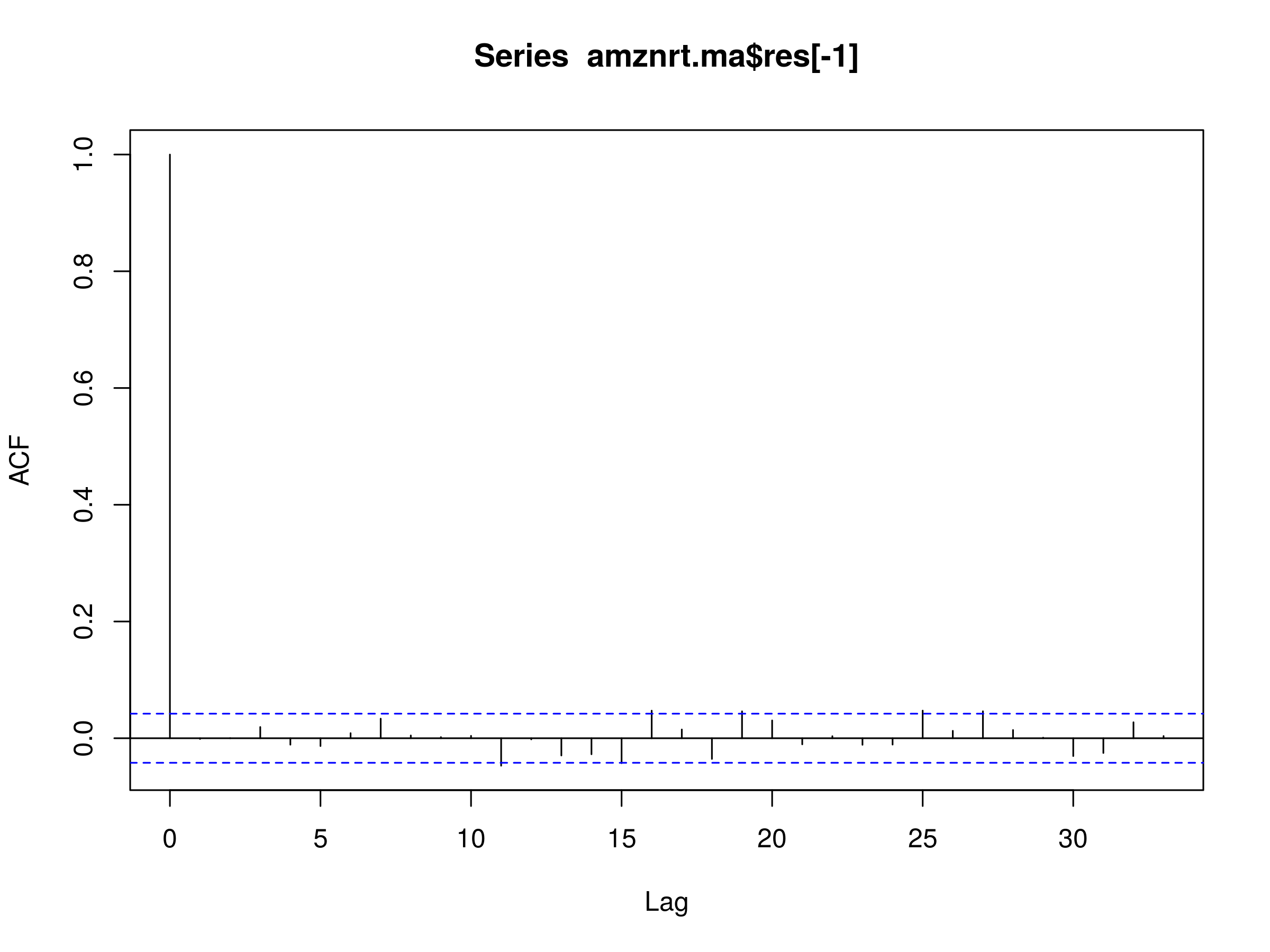
> acf(amznrt.ma$res[-1])
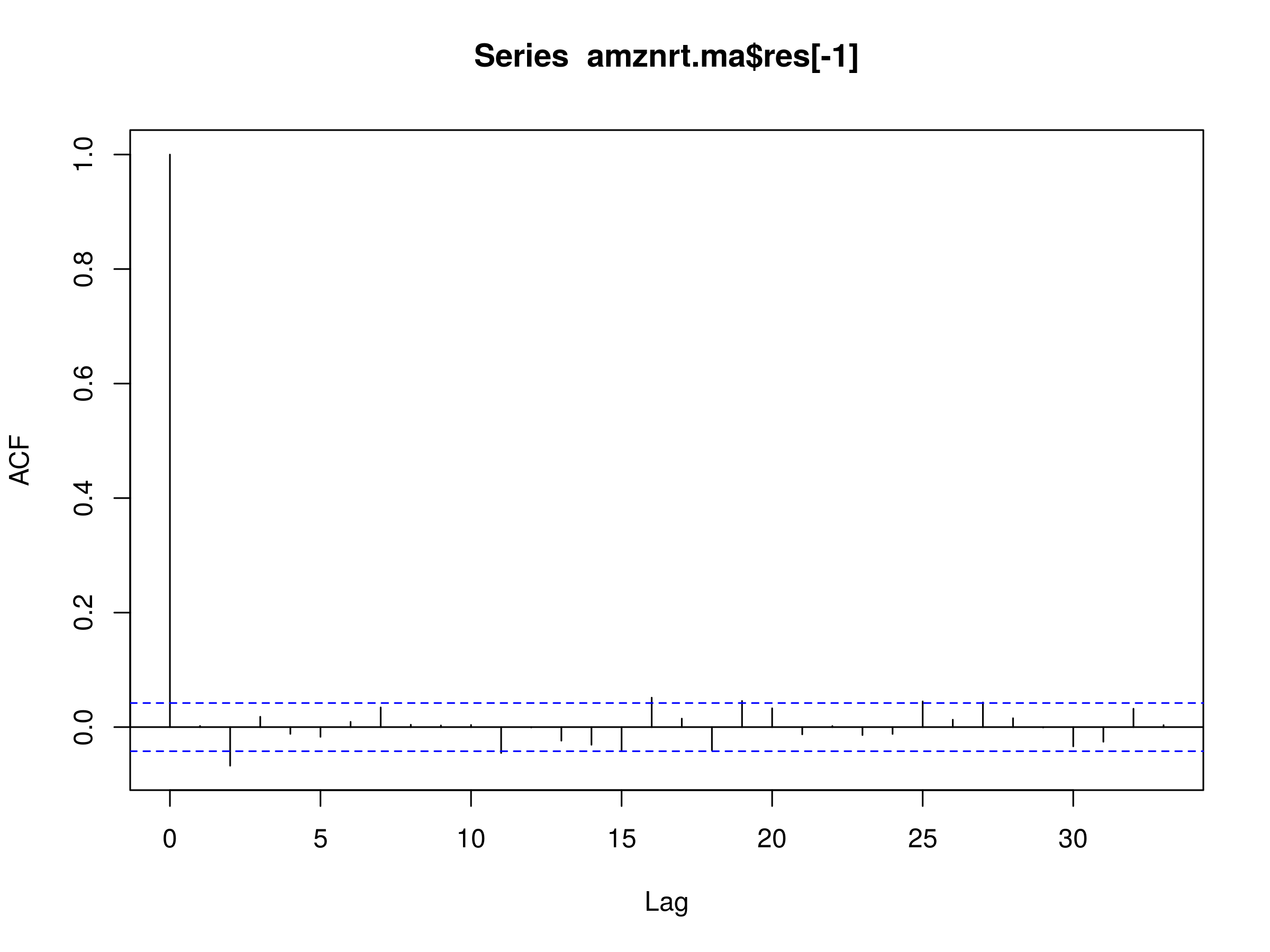 Residuals of MA(1) Model Fitted to AMZN Daily Log Prices
Notice that we have a few significant peaks at lags $k=2$, $k=11$, $k=16$ and $k=18$, indicating that the MA(1) model is unlikely to be a good fit for the behaviour of the AMZN log returns, since this does not look like a realisation of white noise.
Let's try a MA(2) model:
> amznrt.ma <- arima(amznrt, order=c(0, 0, 2))
> amznrt.ma
Call:
arima(x = amznrt, order = c(0, 0, 2))

Coefficients:
          ma1      ma2  intercept
      -0.0254  -0.0689     0.0012
s.e.   0.0215   0.0217     0.0005

sigma^2 estimated as 0.0007011:  log likelihood = 4801.02,  aic = -9594.05
Both of the estimates for the $\beta$ coefficients are negative. Let's plot the residuals once again:
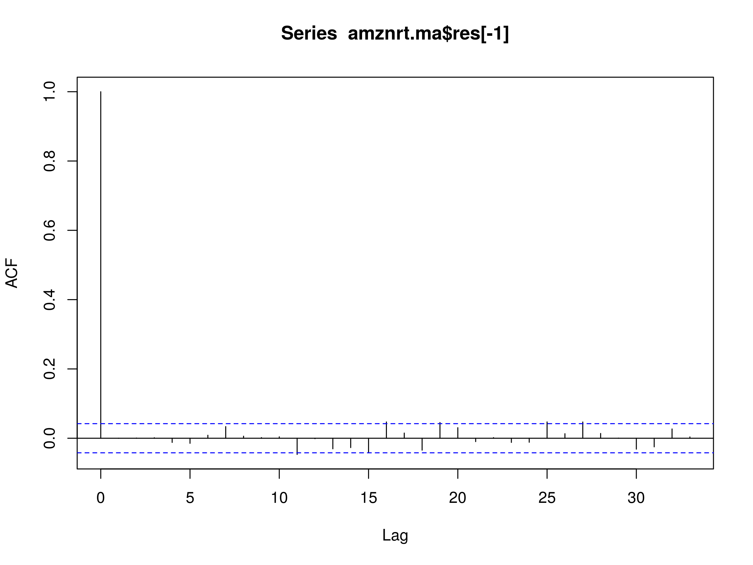
> acf(amznrt.ma$res[-1])
 Residuals of MA(2) Model Fitted to AMZN Daily Log Prices
We can see that there is almost zero autocorrelation in the first few lags. However, we have five marginally significant peaks at lags $k=12$, $k=16$, $k=19$, $k=25$ and $k=27$. This is suggestive that the MA(2) model is capturing a lot of the autocorrelation, but not all of the long-memory effects. How about a MA(3) model?
> amznrt.ma <- arima(amznrt, order=c(0, 0, 3))
> amznrt.ma
Call:
arima(x = amznrt, order = c(0, 0, 3))

Coefficients:
          ma1      ma2     ma3  intercept
      -0.0262  -0.0690  0.0177     0.0012
s.e.   0.0214   0.0217  0.0212     0.0005

sigma^2 estimated as 0.0007009:  log likelihood = 4801.37,  aic = -9592.75
Once again, we can plot the residuals:
> acf(amznrt.ma$res[-1])
 Residuals of MA(3) Model Fitted to AMZN Daily Log Prices
The MA(3) residuals plot looks almost identical to that of the MA(2) model. This is not surprising, as we're adding a new parameter to a model that has seemingly explained away much of the correlations at shorter lags, but that won't have much of an effect on the longer term lags.
All of this evidence is suggestive of the fact that an MA(q) model is unlikely to be useful in explaining all of the serial correlation in isolation, at least for AMZN.
S&P500
If you recall, in Part 1 we saw that the first order differenced daily log returns structure of the S&P500 possessed many significant peaks at various lags, both short and long. This provided evidence of both conditional heteroskedasticity (i.e. volatility clustering) and long-memory effects. It lead us to conclude that the AR(p) model was insufficient to capture all of the autocorrelation present.
As we've seen above the MA(q) model was insufficient to capture additional serial correlation in the residuals of the fitted model to the first order differenced daily log price series. We will now attempt to fit the MA(q) model to the S&P500.
One might ask why we are doing this is if we know that it is unlikely to be a good fit. This is a good question. The answer is that we need to see exactly how it isn't a good fit, because this is the ultimate process we will be following when we come across much more sophisticated models, that are potentially harder to interpret.
Let's begin by obtaining the data and converting it to a first order differenced series of logarithmically transformed daily closing prices as in the previous article:
> getSymbols("^GSPC")
> gspcrt = diff(log(Cl(GSPC)))
We are now going to fit a MA(1), MA(2) and MA(3) model to the series, as we did above for AMZN. Let's start with MA(1):
> gspcrt.ma <- arima(gspcrt, order=c(0, 0, 1))
> gspcrt.ma
Call:
arima(x = gspcrt, order = c(0, 0, 1))

Coefficients:
          ma1  intercept
      -0.1284      2e-04
s.e.   0.0223      3e-04

sigma^2 estimated as 0.0001844:  log likelihood = 6250.23,  aic = -12494.46
Let's make a plot of the residuals of this fitted model:
> acf(gspcrt.ma$res[-1])
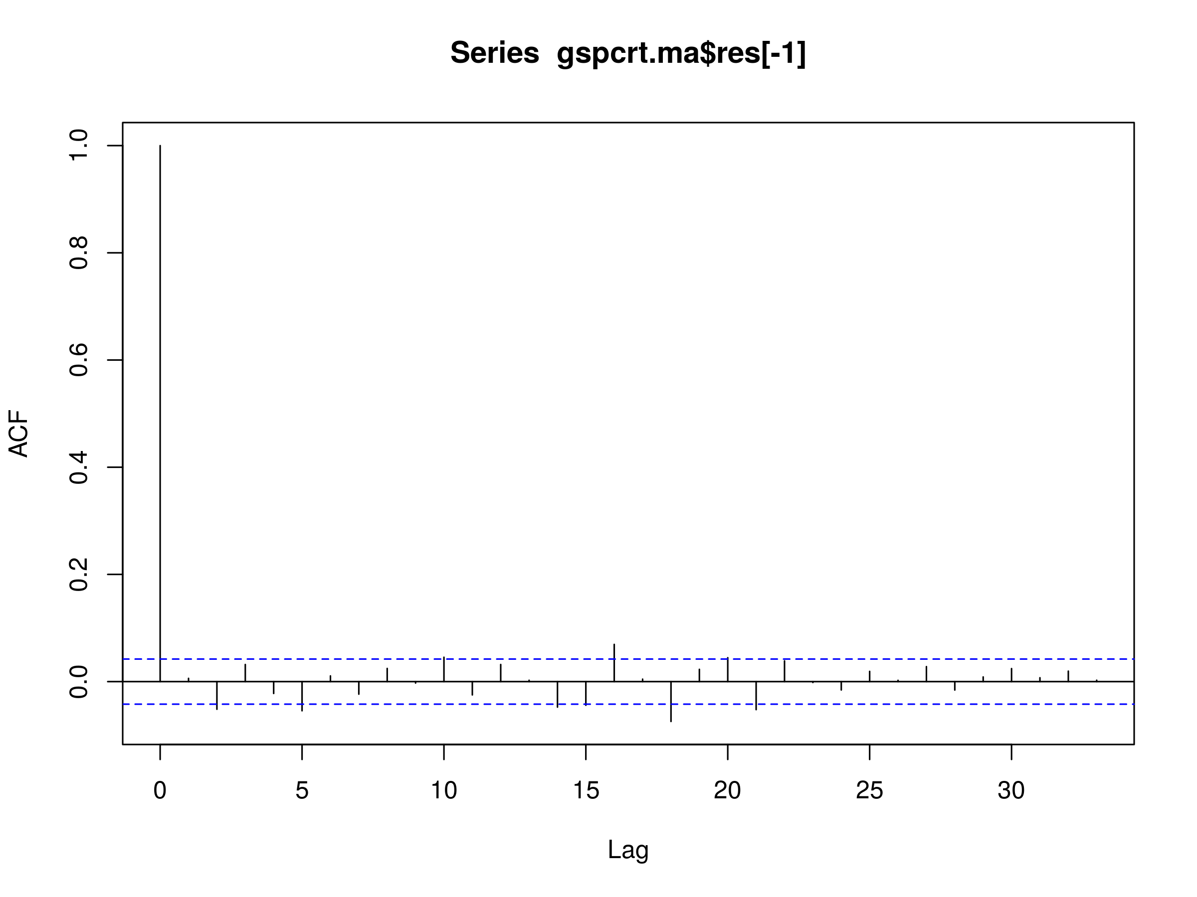 Residuals of MA(1) Model Fitted to S&P500 Daily Log Prices
The first significant peak occurs at $k=2$, but there are many more at $k \in \{ 5, 10, 14, 15, 16, 18, 20, 21 \}$. This is clearly not a realisation of white noise and so we must reject the MA(1) model as a potential good fit for the S&P500.
Does the situation improve with MA(2)?
> gspcrt.ma <- arima(gspcrt, order=c(0, 0, 2))
> gspcrt.ma
Call:
arima(x = gspcrt, order = c(0, 0, 2))

Coefficients:
          ma1      ma2  intercept
      -0.1189  -0.0524      2e-04
s.e.   0.0216   0.0223      2e-04

sigma^2 estimated as 0.0001839:  log likelihood = 6252.96,  aic = -12497.92
Once again, let's make a plot of the residuals of this fitted MA(2) model:
> acf(gspcrt.ma$res[-1])
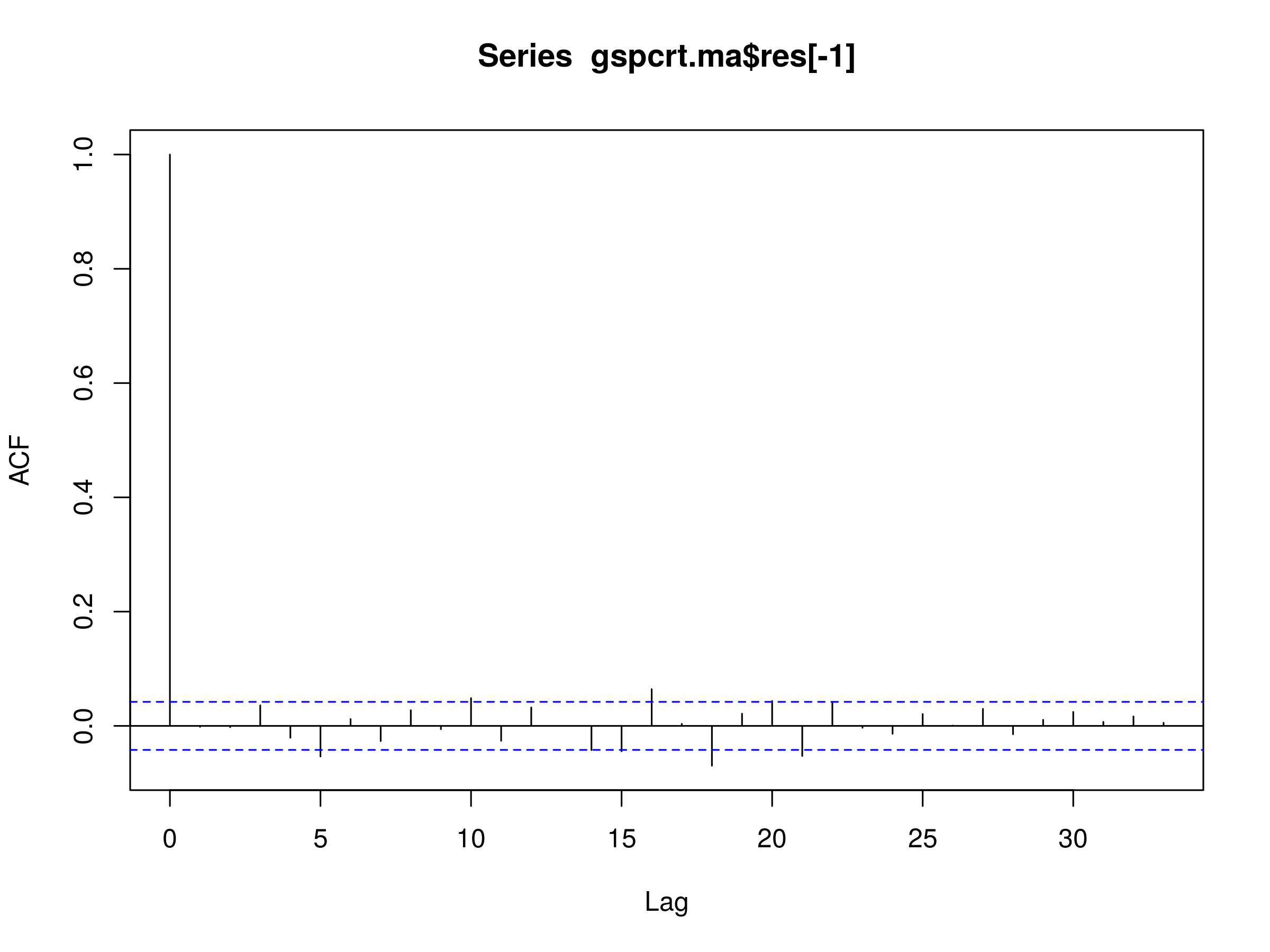 Residuals of MA(2) Model Fitted to S&P500 Daily Log Prices
While the peak at $k=2$ has disappeared (as we'd expect), we are still left with the significant peaks at many longer lags in the residuals. Once again, we find the MA(2) model is not a good fit.
We should expect, for the MA(3) model, to see less serial correlation at $k=3$ than for the MA(2), but once again we should also expect no reduction in further lags.
> gspcrt.ma <- arima(gspcrt, order=c(0, 0, 3))
> gspcrt.ma
Call:
arima(x = gspcrt, order = c(0, 0, 3))

Coefficients:
          ma1      ma2     ma3  intercept
      -0.1189  -0.0529  0.0289      2e-04
s.e.   0.0214   0.0222  0.0211      3e-04

sigma^2 estimated as 0.0001838:  log likelihood = 6253.9,  aic = -12497.81
Finally, let's make a plot of the residuals of this fitted MA(3) model:
> acf(gspcrt.ma$res[-1])
 Residuals of MA(3) Model Fitted to S&P500 Daily Log Prices
This is precisely what we see in the correlogram of the residuals. Hence the MA(3), as with the other models above, is not a good fit for the S&P500.
Next Steps
We've now examined two major time series models in detail, namely the Autogressive model of order p, AR(p) and then Moving Average of order q, MA(q). We've seen that they're both capable of explaining away some of the autocorrelation in the residuals of first order differenced daily log prices of equities and indices, but volatility clustering and long-memory effects persist.
It is finally time to turn our attention to the combination of these two models, namely the Autoregressive Moving Average of order $p,q$, ARMA(p,q) to see if it will improve the situation any further.
However, we will have to wait until the next article for a full discussion!