In this article we will explore simulation of Brownian Motions, one of the most fundamental concepts in derivatives pricing. Brownian Motion is a mathematical model used to simulate the behaviour of asset prices for the purposes of pricing options contracts.
A typical means of pricing such options on an asset, is to simulate a large number of stochastic asset paths throughout the lifetime of the option, determine the price of the option under each of these scenarios, average these prices, then discount this average to produce a final price. This is an example of a Monte Carlo method.
This article will focus specifically on simulating Brownian Motion paths using the Python programming language. It will begin by looking at Standard Brownian Motion, then will proceed to add more complexity to the Brownian Motion dynamics. As always with every QuantStart article full code to completely replicate the exact results below will be provided.
The article is heavily influenced by the highly recommended text of Monte Carlo Methods for Financial Engineering by Paul Glasserman [Glasserman, 2003]. This book covers the necessary theoretical detail that leads to the discretisation formulae that are presented (without derivation) below.
The article will begin by simulating the so-called "Standard" Brownian Motion, which involves Brownian Motion paths with zero mean and unit variance. It will then discuss how to include a non-zero constant mean and non-unit constant variance for Brownian Motion path simulation. In future articles we will discuss time-varying mean and variance dynamics, initially with piecewise constant mean and variance and subsequently simulation with fully time-varying mean and variance.
Note: If you would like a mathematical recap of how Brownian Motion is defined then please refer to our previous article on the topic here.
Standard Brownian Motion
The following equation is taken from Equation 3.2 in [Glasserman, 2003]. It provides a recursion relation for a (single) Brownian Motion path across $n$ points (not necessarily equally distributed in time). The relation essentially says that the new Brownian Motion path value at time $t_{i+1}$ is equal to the value at $t_i$ (i.e. one value previously) plus the square root of the time difference between each value multiplied by the normally distributed sample at time $t_{i+1}$.
\begin{eqnarray} W(t_{i+1}) = W(t_i) + \sqrt{t_{i+1} - t_i} Z_{i+1} \end{eqnarray}However, we are going to utilise the vectorised approach of the Python NumPy library to generate $k$ paths concurrently. To achieve this we will sample $k \times n$ draws from a standard normal distribution, then utilise these in $k$ vectorised path simulations through the use of the recursion relation above.
The first task is to import the relevant quantitative and visualisation libraries needed for the subsequent analysis. This includes Matplotlib, NumPy, Pandas and Seaborn:
import matplotlib.pyplot as plt
import numpy as np
import pandas as pd
import seaborn as sns
We also need to set a random seed value to ensure that your values exactly match ours. For this we need to utilise a (pseudo-)Random Number Generator (RNG), which in this case is the default provided by NumPy. Then it is necessary to provide an integer seed value to ensure reproducibility of all results below:
rng = np.random.default_rng(42)
The next step is to choose the number of paths and the number of time steps per path. We have specified $k=50$ paths, each with $n=1000$ time steps:
paths = 50
points = 1000
Since this is a standard Brownian Motion the drift (mean) of the process is zero, while the volatility (standard deviation) is unity:
mu, sigma = 0.0, 1.0
The next step is to draw all of the necessary samples from a standard normal (Gaussian) distribution and store them in a matrix with paths rows and points columns ($k \times n$ values). For this we utilise the same RNG as above, since it is seeded for reproducibility:
Z = rng.normal(mu, sigma, (paths, points))
The next step is to specify the time interval over which the simulation occurs. We will utilise the interval $[0.0, 1.0]$. We will also restrict ourselves, for the purpose of this tutorial, to using equal step sizes, denoted by $\Delta t = t_{i+1} - t_i$. For this we simply divide the interval length by the number of time points minus one:
interval = [0.0, 1.0]
dt = (interval[1] - interval[0]) / (points - 1)
In order to produce a plot in Matplotlib it is necessary to create a "linear space" axis. The following simply takes the interval and creates points numbers of equally space points (inclusive of the start and end value of the interval) in an array, which will be used as our "time axis":
t_axis = np.linspace(interval[0], interval[1], points)
The following code implements the recursion formula (3.2) from [Glasserman, 2003]. We initially create a $k \times n$ size matrix W to store the Brownian Motion path results full of zeros. Then we loop over the number of points in the time axis. For each of these points we use NumPy vectorised notation (W[:, real_idx]) to set the next path values, for each path, equal to the previous path value plus the square root of the time step $\Delta t$ multiplied by the appropriate standard normal samples within the Z matrix:
W = np.zeros((paths, points))
for idx in range(points - 1):
    real_idx = idx + 1
    W[:, real_idx] = W[:, real_idx - 1] + np.sqrt(dt) * Z[:, idx]
We can then use Matplotlib to plot all of these paths on the same figure. For this we use the subplots method, which allows us more fine-grained control of how the figure and axis is configured. We specify that we want a single row and column, then provide a figure size in inches (at a default resolution of 100 dots-per-inch (dpi)). Then we loop over the number of paths and plot the time axis against the appropriate row in the W matrix, using the NumPy vectorised notation (W[path, :]). Finally, we plot the figure:
fig, ax = plt.subplots(1, 1, figsize=(12, 8))
for path in range(paths):
    ax.plot(t_axis, W[path, :])
ax.set_title("Standard Brownian Motion sample paths")
ax.set_xlabel("Time")
ax.set_ylabel("Asset Value")
plt.show()
This produces the following image:
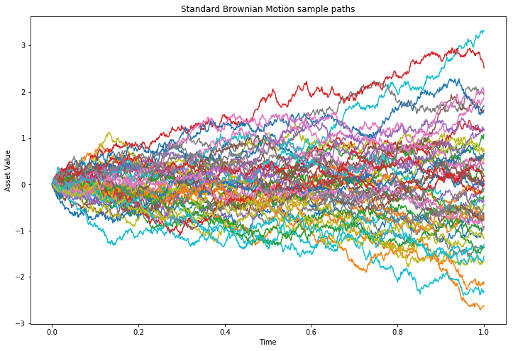
It is fairly clear that the bulk of the paths are clustering around zero near $t=1.0$ (the end of the simulation), within the -1 and 1 values, while there are a few examples of more extreme ending values. This is the expected behaviour for a standard Brownian Motion.
However, this can be made more quantitative by estimating the distribution of final path values for each of the $k=50$ sample paths produced. To achieve this we can use a Kernel Density Estimate (KDE), which is a method for estimating a (continuous) probability distribution from finite sample data. The Seaborn statistical visualisation library will be used for this.
The first step is to create a Pandas DataFrame (with a single column) of the sample path ending values:
final_values = pd.DataFrame({'final_values': W[:, -1]})
Then we can use Seaborn to estimate and plot a KDE distribution of the final values:
fig, ax = plt.subplots(1, 1, figsize=(12, 8))
sns.kdeplot(data=final_values, x='final_values', fill=True, ax=ax)
ax.set_title("Kernel Density Estimate of asset path final value distribution")
ax.set_ylim(0.0, 0.325)
ax.set_xlabel('Final Values of Asset Paths')
plt.show()
This produces the following image:
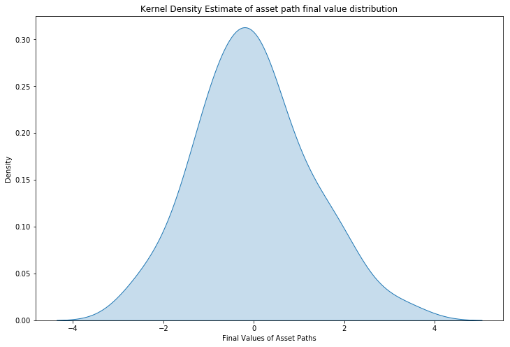
As can be seen this looks somewhat like a standard normal distribution (i.e. mean zero, standard deviation unity). However, we can also calculate the sample mean and standard deviation of this distribution:
print(final_values.mean(), final_values.std())
This produces the following output:
(final_values   -0.011699
 dtype: float64,
 final_values    1.251382
 dtype: float64)
The mean of -0.01 is close to zero and the standard deviation of 1.25 is fairly close to unity. If more paths were calculated these values would tend to that of a standard normal distribution, due to the law of large numbers.
In the next section we are going to allow a non-zero mean and non-unit standard deviation for the sampling paths.
Constant Drift and Volatility Brownian Motion
The next recursion relation is taken from Equation 3.3 from [Glasserman, 2003]. It is a modification from the equation above to include an additional term $\mu (t_{i+1} - t_i)$ along with the multiplication of the final term by $\sigma$. This is what allows a non-zero mean, as well as a non-unit standard deviation:
\begin{eqnarray} X(t_{i+1}) = X(t_i) + \mu (t_{i+1} - t_i) + \sigma \sqrt{t_{i+1} - t_i} Z_{i+1} \end{eqnarray}Much of the code and calculated variables from the previous section can be completely re-used, including the (random seeded) standard normal draws matrix, Z. It is necessary to set the new drift mu_c and volatility sigma_c, which we have set to 5 and 2 respectively:
mu_c, sigma_c = 5.0, 2.0
The following code implements Equation 3.3 from [Glasserman, 2003]. Notice the inclusion of mu_c * dt as well as the inclusion of sigma_c * ... to the latter term. It is still possible to use $\Delta t = t_{i+1} - t_i$ (dt) since we are only using constant length timesteps:
X = np.zeros((paths, points))
for idx in range(points - 1):
    real_idx = idx + 1
    X[:, real_idx] = X[:, real_idx - 1] + mu_c * dt + sigma_c * np.sqrt(dt) * Z[:, idx]
As with the standard Brownian Motion we can plot the collection of sample paths produced:
fig, ax = plt.subplots(1, 1, figsize=(12, 8))
for path in range(paths):
    ax.plot(t_axis, X[path, :])
ax.set_title("Constant mean and standard deviation Brownian Motion sample paths")
ax.set_xlabel("Time")
ax.set_ylabel("Asset Value")
plt.show()
This produces the following image:
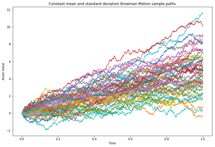
Notice the positive drift towards a mean of 5, with an increased spread compared to the standard Brownian Motion. It is also possible to vary the values of mu_c and sigma_c to produce different path dynamics.
Next Steps
In the next article in the series we will relax the assumption of constant mean and standard deviation, allowing for a time-varying mean and standard deviation to introduce more sophisticated asset dynamics. In future articles we will consider multi-dimensional Brownian Motion, the "Brownian Bridge" and Geometric Brownian Motion.
References
- [Glasserman, 2003] - Glasserman, P. (2003) Monte Carlo Methods in Financial Engineering, Springer.
Full Code
# Imports
import matplotlib.pyplot as plt
import numpy as np
import pandas as pd
import seaborn as sns

# Seed the random number generator
rng = np.random.default_rng(42)

# Determine the number of paths and points per path
points = 1000
paths = 50

# Create the initial set of random normal draws
mu, sigma = 0.0, 1.0
Z = rng.normal(mu, sigma, (paths, points))

# Define the time step size and t-axis
interval = [0.0, 1.0]
dt = (interval[1] - interval[0]) / (points - 1)
t_axis = np.linspace(interval[0], interval[1], points)

# Use Equation 3.2 from [Glasserman, 2003] to sample 50 standard brownian motion paths
W = np.zeros((paths, points))
for idx in range(points - 1):
    real_idx = idx + 1
    W[:, real_idx] = W[:, real_idx - 1] + np.sqrt(dt) * Z[:, idx]

# Plot these paths
fig, ax = plt.subplots(1, 1, figsize=(12, 8))
for path in range(paths):
    ax.plot(t_axis, W[path, :])
ax.set_title("Standard Brownian Motion sample paths")
ax.set_xlabel("Time")
ax.set_ylabel("Asset Value")
plt.show()

# Obtain the set of final path values
final_values = pd.DataFrame({'final_values': W[:, -1]})

# Estimate and plot the distribution of these final values with Seaborn
fig, ax = plt.subplots(1, 1, figsize=(12, 8))
sns.kdeplot(data=final_values, x='final_values', fill=True, ax=ax)
ax.set_title("Kernel Density Estimate of asset path final value distribution")
ax.set_ylim(0.0, 0.325)
ax.set_xlabel('Final Values of Asset Paths')
plt.show()

# Output the mean and stdev of these final values
print(final_values.mean(), final_values.std())

# Create a non-zero mean and non-unit standard deviation
mu_c, sigma_c = 5.0, 2.0

# Use Equation 3.3 from [Glasserman, 2003] to sample 50 brownian motion paths
X = np.zeros((paths, points))
for idx in range(points - 1):
    real_idx = idx + 1
    X[:, real_idx] = X[:, real_idx - 1] + mu_c * dt + sigma_c * np.sqrt(dt) * Z[:, idx]

# Plot these paths
fig, ax = plt.subplots(1, 1, figsize=(12, 8))
for path in range(paths):
    ax.plot(t_axis, X[path, :])
ax.set_title("Constant mean and standard deviation Brownian Motion sample paths")
ax.set_xlabel("Time")
ax.set_ylabel("Asset Value")
plt.show()